CST同轴线器件的仿真设计分析—CST2013设计实例

    A key feature of CST MICROWAVE STUDIO is the Complete Technology approach that allows a simulator or mesh type that is best suited to a particular problem.  Another benefit is the ability to compare the results obtained by completely independent approaches.  We demonstrate this strength in the following two sections by calculating the S-Parameters with the transient solver as well as the frequency domain solver.  The transient simulation uses a hexahedral mesh while the frequency domain calculation is performed with a tetrahedral mesh.  Both sections are self-contained parts and it is sufficient to work through only one of them, depending on what solver you are interested in.  The chapter ends with a comparison of the two methods.

    Please note that not all solvers may be available to you due to license restrictions. Please contact your sales office for more information.

    Transient Solver

    Frequency Range Considerations for the Transient Solver

    In contrast to frequency domain tools, a transient solvers performance can be degraded if the frequency range is chosen to be too small (the opposite is usually true for frequency domain solvers).

    We recommend using reasonably large bandwidths of 20% to 100% for the transient simulation.  In this example, the S-Parameters are to be calculated for a frequency range between 0 and 8 GHz.  With the center frequency being 4 GHz, the bandwidth (8 GHz - 0 GHz = 8 GHz) is 200% of the center frequency, which is acceptable.  Thus, you can simply choose the desired frequency range between 0 and 8 GHz.

   Please note: Assuming that you are interested primarily in a frequency range of e.g. 11.5 to 12.5 GHz (for a narrow band filter), then the bandwidth would only be about 8.3%.  In this case, it is logical to increase the frequency range (without losing accuracy) to a bandwidth of 30%, which corresponds to a frequency range of 10.2 to 13.8 GHz.  This extension of the frequency range could speed up your simulation by more than a factor of three!

    The lower frequency can be set to zero without any problems.  The calculation time can often be reduced by half if the lower frequency is set to zero rather than e.g. 0.01 GHz.

    Transient Solver Settings

    The solvers parameters are specified in the Transient Solver Parameters dialog box that can be opened by selecting Home: Simulation > Start Simulation > Time Domain Solver .

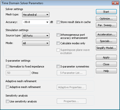
    Because this two port structure is lossless, the transient solver will need to calculate only a single port  to obtain the full S-matrix, even if you specify All Ports for the Source type.

    In this case, you can keep the default settings and press the Start button to start the calculation. When the simulation has finished or has been aborted, both items disappear.  During the simulation, the Message Window will show some details about the performed simulation.

    Transient Solver Results 

    Congratulations, you have simulated the coaxial connector using the transient solver! Lets look at the results:

    1D Results (Port Signals, S-Parameters)

    First, observe the port signals.  Open the 1D Results folder in the navigation tree and click on the Port signals folder.

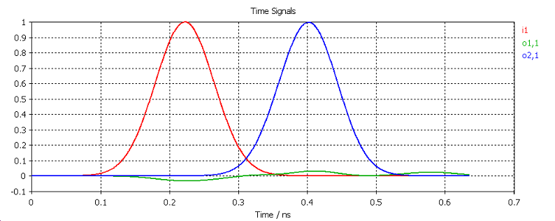
    This plot shows the incident, reflected and transmitted wave amplitudes at the ports versus time.  The incident wave amplitude is called i1 and the reflected or transmitted wave amplitudes of the two ports are o1,1 and o2,1.  These curves show the delay in the transition from the input port to the output port and a relatively small reflection at the input port.

    The S-Parameters can be plotted by clicking on the 1D Results  S-Parameters folder in the navigation tree.

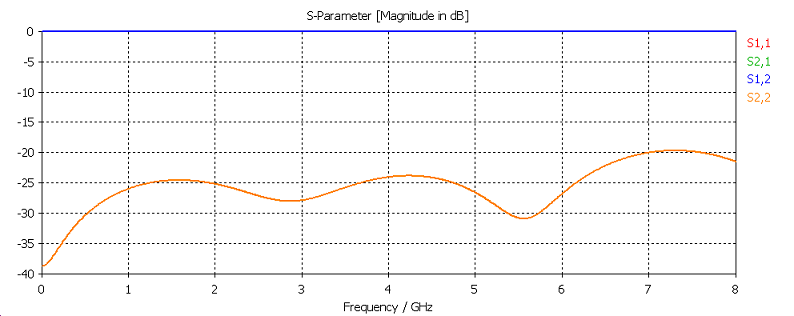
    As expected, the input reflection S1,1 is quite small across the entire frequency range.

    2D and 3D Results (Port Modes and Field Monitors)

    Finally, you can observe the 2D and 3D field results.  You should first inspect the port modes that can be easily displayed by opening the 2D/3D Results  Port Modes  Port1 folder from the navigation tree.  To visualize the electric field of the port mode, please click on the e1 folder.  After properly rotating the view you should obtain a plot similar to the following picture:

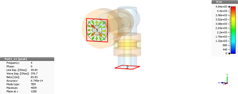
    The plot also displays some important properties of the mode, such as mode type, propagation constant and line impedance.  The port mode at the second port can be visualized in the same manner.

    The three-dimensional surface current distribution on the conductors can be shown by selecting one of the entries in the 2D/3D Results  Surface Current folder from the navigation tree.  The surface current at a frequency of 2 GHz can thus be visualized by clicking at the 2D/3D Results  Surface Current  surface current (f=2) [1] entry:

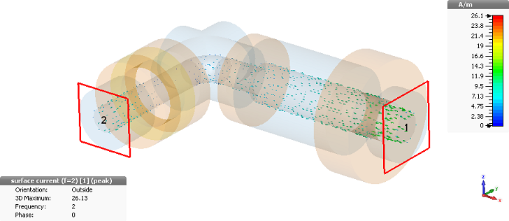
    You can toggle an animation of the currents on and off by selecting the Result Tools  2D/3D Plot  Animate Fields item.  The surface currents for the other frequencies can be visualized in the same manner.

上一页  [1] [2] [3] [4] [5] [6] [7] [8] [9] [10] 下一页