CST同轴线器件的仿真设计分析—CST2013设计实例

     Before you start the solver, you should always check the boundary and symmetry conditions.  This is most easily accomplished by entering the boundary definition mode by selecting Simulation: Settings  Boundaries .  The boundary conditions will then become visualized in the main view as follows:

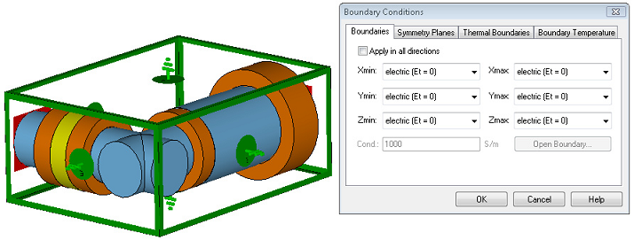
     Here, all boundary conditions are set to electric which means that the structure is embedded in a perfect electrically conducting housing.  These defaults are appropriate for this example.

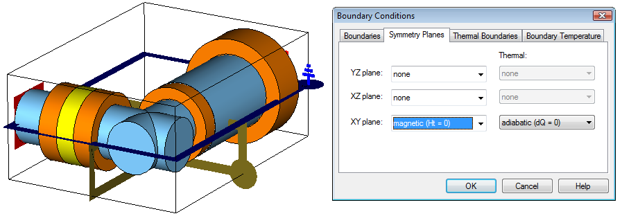
     Due to the structures symmetry to the XY plane and the fact that the magnetic field in the coaxial cable is perpendicular to this plane, a symmetry condition can be used.  This symmetry reduces the time required for the simulation by a factor of two.

    Please enter the symmetry plane definition mode by activating the Symmetry Planes tab in the dialog box.  By setting the symmetry plane XY to magnetic, you force the solver to calculate only the modes that have no tangential magnetic field component on these planes (thereby forcing the electric field to be tangential to these planes).The screen should then look as follows:

     Please note that you also could double-click on the symmetry planes handle and choose the proper symmetry condition from the context menu.

    Finally, press the OK button to complete this step.

    In general, you should always make use of symmetry conditions whenever possible to reduce calculation times by a factor of two to eight.

     Define the Frequency Range

     The frequency range for the simulation should be chosen with care.  Different considerations must be made when using a transient solver or a frequency domain solver (see next chapter for details).

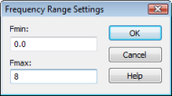
    For this example, we will choose a frequency range from 0 to 8 GHz.  Open the frequency range dialog box Simulation: Settings  Frequency  and enter the range of 0 to 8 (GHz) before pressing the OK button (the frequency unit has previously been set to GHz and is displayed in the status bar):

    Define Field Monitors

    CST MICROWAVE STUDIO uses the concept of monitors to specify which field data to store.  In addition to choosing the type, you can also specify whether the field is recorded at a fixed frequency or at a sequence of time samples (the latter case applies only to the transient solver).  You may define as many monitors as necessary to obtain the fields at various frequencies.  For the transient solver, all monitors are calculated from a single simulation run by the Fourier Transform.  Consequently, the computational overhead for a defined monitor is relatively small.

    Please note that an excessive number of field monitors may significantly increase the memory space required for the simulation.

    Assume that you are interested in the current distribution on the coaxial cables conductors at several frequencies (2, 4, 6 and 8 GHz).  To add field monitors, select Simulation: Monitors > Field Monitor . 

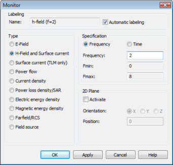
    In this dialog box, you should first select the Type H-Field/Surface current before specifying the frequency for the monitor in the Frequency field.  Afterwards, press the Apply button to store the monitors data.  Please define monitors for the following frequencies: 2, 4, 6, 8 (with GHz being the currently active frequency unit).  Please make sure that you press the Apply button for each monitor (the monitor definition is then added in the Monitors folder in the navigation tree).

    After the monitor definition is completed, you can close this dialog box by pressing the OK button.

上一页  [1] [2] [3] [4] [5] [6] [7] [8] [9] [10] 下一页