This help page provides an overview of the particle sources and the emission models for the tracking and the PIC solvers.
Tracking source emission models
Kinetic settings (common for all tracking emission models)
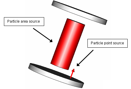
To create a particle source, the geometrical properties of the emission, such as the shape of the emission area or the arrangement of the emission points, must be defined. For example, particle sources can be assigned to an area of either a PEC (perfect electrical conductor) or a non-PEC solid, they can be a single emission point or the aggregate of many emission points distributed homogeneously on a circular area .
Note:
The relation between the macro particles charge (dQ) and the current density (J) is determined by the initial time step (dt) of the tracking simulation and the assigned area (A) of the starting point.
![]()
Together with the starting-triangle’s area, the complete current of the source can be computed by integrating the current density over the emitting area.
Selection of an emitting
face
Note that the emitting face can be located on either a PEC-solid or
a solid with an arbitrary material definition.
Triangulation of
the chosen face
The emission points of the particles are the center points of the triangles.
The resolution of the triangulation grid can be model-oriented (sufficient
triangles to reconstruct the face within a certain accuracy) or mesh-oriented.
Selecting the checkbox ”Adjust density to mesh” leads to a
emission density which guarantees even in its worst setting a density
of one or more emission point(s) in each emitting mesh cell. So selecting
the ”Adjust density to mesh” option is highly recommended
for an accurate modeling of the physical emission process.
Definition of the condition
of extraction
The tracking solver and the PIC solver contain different sets of emission
models, which will be described in the following sections.
Selection of an emitting
point by using the point pick tool (optional)
Before activating the particle point source tool one can define the
start position by activating one of the point pick tools which are available
via Modeling:
Picks![]() Pick Point.
Pick Point.
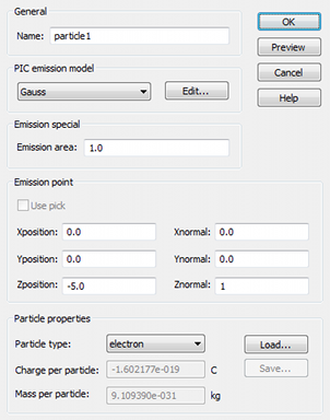
Assigning a current emitting
area to a point source.
For a couple of emission models it is necessary to define a virtual
emitting area, so that the emission model can compute charge distributions
and current densities.
Definition of the condition
of extraction
The tracking solver and the PIC solver contain different sets of emission
models, which will be described in the following sections.
Selection of an emitting
circular surface by using the area- or edge- pick tool (optional)
The face- or edge pick tools which are available
via Modeling:
Picks![]() Pick can
be used to define the circular emitting area. It is also possible to define
a circular face inside the particle source dialog box after the pick tool
has been activated ; to skip this mode simply press the Enter key. Inside
the dialog box, one can visualize the emission point arrangement and emission
direction, by using the Preview button. By checking the box Invert picked normal , one can invert the emission direction.
Pick can
be used to define the circular emitting area. It is also possible to define
a circular face inside the particle source dialog box after the pick tool
has been activated ; to skip this mode simply press the Enter key. Inside
the dialog box, one can visualize the emission point arrangement and emission
direction, by using the Preview button. By checking the box Invert picked normal , one can invert the emission direction.
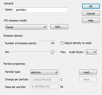
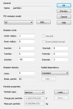
Assigning a particle emission
density to the source.
The number of emitted particles can be adjusted with the Lines
parameter which controls the number of emission points per unit area.
By clicking the Preview button, one can visualize the distribution
of the emission points on the circular emission area inside the main view.
The number of emission points is shown inside the dialog box.
Define
a radial dependency for the emitted current.
For circular sources it is possible to preset
a radial dependency for the emitted current. A radial distribution function
can be selected from the corresponding dropdown list and its parameters
can be adjusted to suit the modeling needs for the emitted current. Not
for all emission models is such a radial dependency presetting meaningful.
In particular, the non-constant radial dependencies apply only for the
Gauss (PIC), DC (PIC) and Fixed (TRK) emission models. Detailed information
about the radial dependency parameters can be found in Circular
Distribution Functions help page.
Definition of the condition
of extraction
The tracking solver and the PIC solver contain different sets of emission
models, which will be described in the following sections.
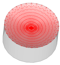
An example of a circular source with a finite inner radius is shown below. Here, the parameter Lines is set to 3. The blue dots represent the emission points and the arrow represents the source normal.
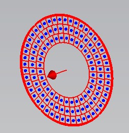
More information about the circular source settings can be found in the Particle Circle Source help page.
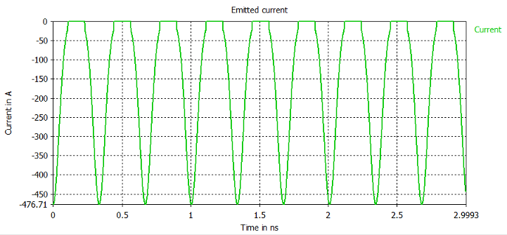
In PIC simulations,
the emitted power and current of particle sources can be viewed as a function
of time. The results are available in the Navigation
Tree: 1D Results![]() Emission Information result folder.
Emission Information result folder.
Tracking Emission Models Overview
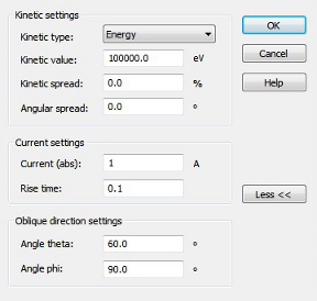
For simulations with the tracking solver, a number of settings must be specified. The emission models share a common kinetic part where the so-called kinetic settings, e.g. the emission energy, can be specified. These settings are described in the section:
The rest of the settings deals with the way the emitted current is prescribed or calculated. This gives rise to several emission models :
There are two models that can be chosen to define the kinetic settings. One possibility is the so-called uniform distribution model, in which a user-selected particle physical quantity, such as energy, follows a uniform distribution. The second possibility is the Maxwell-Boltzmann distribution, where the statistical properties of the emitted particles depend on a given temperature.
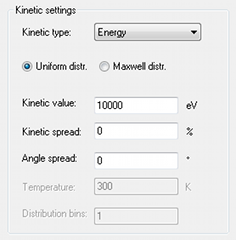
Uniform distribution
In the uniform distribution model, the physical quantity that is distributed uniformly, the so-called kinetic type, must be selected. The following types are available:
|
Velocity |
|
|
Velocity in terms of speed of light |
|
|
Lorentz factor |
|
|
Normalized momentum |
|
|
Energy |
|
|
Temperature |
|
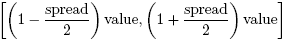
An energy spread parameter introduces the energy spread as a percentage of the given mean-value. If the emitted current is prescribed (either as absolute value or as current-density setting), the charge of the particles is treated adequately. The kinetic emission type (e.g. energy, momentum) is calculated uniformly distributed in the range of:
The kinetic spread is always applied to the selected kinetic type. This means that a kinetic spread of 10% applied to a Beta value leads to another energy distribution as if it would be applied to the equivalent momentum value. Here is an example: a beta of 0.9 with 20% spread leads to a range from 0.81 beta to 0.99 beta. This is equivalent to a normalized momentum of 2.065 with a range from 1.381 to 7.018. Note that a uniform beta distribution is not equivalent to a uniform momentum distribution.
Maxwellian thermal velocity distribution
The Maxwellian thermal velocity distribution characterizes the velocity distribution of particles for a given temperature. Its mathematical description is given by:
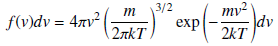
Here f(v) represents the probability of finding particles with the given velocity in the gas. The integral of f(v) from 0 to infinity results to 1. The diagram below shows the velocity distribution of particles for two temperatures of 300K and 900K. In order to project this initial velocity distribution to the emitting particles, so called bins with fixed velocities are defined. The amount of particles in each bin is the same and their velocity is the medium velocity of each bin. The bin distribution samples the Maxwellian thermal velocity distribution thus providing a more physical representation of the initial emission conditions.

Note: The amount of emitted particles does not change, but the start velocity for each particle is randomly chosen from one of the bins.
Angle spread
When this parameter is zero, the particles are emitted along the normal of the source surface, i.e. the angle theta between the emission velocity and the local surface normal at the emission point is zero. However, experiments have shown that in reality the angle theta is randomly distributed. By specifying a finite angle spread, the particles are emitted at random angles around the normal. The maximum angular deviation from the normal is given by the angle spread that is specified by the user. Thus, possible emission vectors lie in a conic region. The axis of this conic region is defined by the normal and the maximum angle between the generatrix (cone's lateral surface) and the axis is given by the angle spread .
In the local spherical coordinate system of a particle, where the Oz axis is defined by the local surface normal, the angle theta (or polar angle) follows a uniform distribution in the interval [0,delta), where delta is the angle spread. The azimuthal angle phi follows a uniform distribution in the interval [0, 360) degrees.
Note: When the oblique emission is active, the angle spread has a slightly different meaning. In this special case, the user is referred to the corresponding oblique emission section for a more detailed description of the effect of the angle spread.
In the fixed emission model, the current carried by the emitted particles is fixed. The user can specify a fixed value either for the current (in A) or for the current density (in A / m²). Unless a finite angular spread is specified in the kinetic settings or the oblique emission model is enabled, the particles are emitted with an initial velocities in the direction of the surface normal.

For circular sources, the oblique emission feature is available as a part of the fixed emission model. By clicking on the More>> button, the user can edit the oblique emission settings.
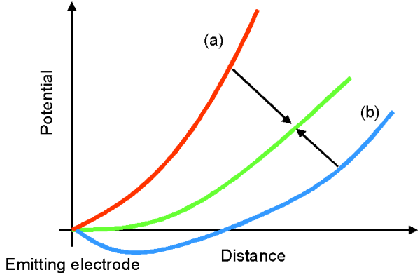
Let's assume that a voltage is applied on two electrodes, one of which, the cathode, can emit charged particles. In the absence of particles, the potential is a linear function of the distance from the emitting electrode (see the green curve of the potential distribution). When particles are present, forming a so-called cloud of space charge, the potential is reduced. This decrease in the potential can be appreciable. The potential profile is depressed as indicated by the dashed red line. As the electron emission rate is increased (by increasing the emitting electrode temperature, for example) the potential is further decreased.
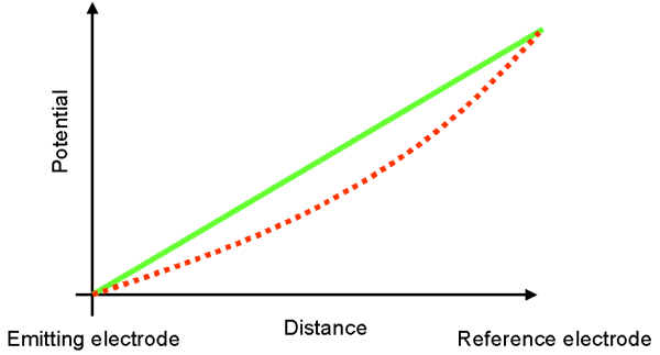
When the electric field at the emitting electrode surface is forced to zero (DF=0) by the particle cloud near the emitting surface, the emission is said to be space charge limited. When a sufficient number of electrons is present so that emission is space charge limited, then the cathode temperature, surface condition etc have no effect on emission. Thus, if a particle source is space charge limited, this limitation dominates over all other emission mechanisms. If the potential difference in front of the surface is larger than zero (case a - red line) additional particles are emitted, so that the stable state (Equilibrium (green line)) will be reached. A reduction of the potential e.g. leads to a potential barrier in front of the particle source (case b, blue line) which suppresses the further extraction of particles, so that also the equilibrium is reached after a short time.
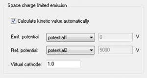
The numerical model describing the space-charge limited emission is based on the Child-Langmuir model. The Child-Langmuir model introduces a virtual electrode at a certain distance d to the emitting surface and measures the potential difference between the electrode and the virtual electrode.
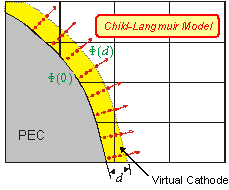
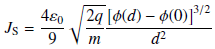
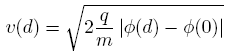
According to the Child-Langmuir law the current density J is emitted at the virtual electrode and the space charge free region is filled up with artificial charges. The divergence model measures the divergence Q of each emitting surface mesh cell and emits particles as long as the divergence results to zero. The start velocity of particles at the surface is zero - at the virtual cathode it can be calculated by:
These space charge limited model parameters are accessible in the dialog box ”Define SCL Emission”:
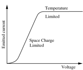
A heated surface emits electrons. A well-known example of such a heated electron-source is a light bulb. The maximum amount of emitted particles is strongly dependent on the temperature of the surface. The thermionic emission model is principally based on the space-charge limited model in combination with a maximal extractable current.
The relationship between the emitted current density J, the specific work function W and the temperature T is given by the Richardson-Dushman equation:
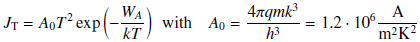
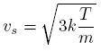
Here q and m denote the particle's charge and mass, k the Boltzmann constant and h the Planck constant. According to the thermionic emission, particles are emitted from surfaces due to their thermionic energy. As temperature is increased, the number of electrons with sufficient energy to escape increases. The start velocity of the emitted particles can be calculated by:
In addition to temperature, the work function of the cathode surface has an extremely strong effect on the rate at which particles are emitted. These parameters are accessible in the ”Define Thermionic Emission” - dialog box:

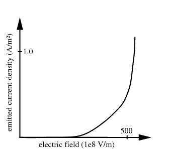
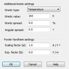
When the electric field that is applied to the surface of a cathode is increased to the level of 10e9 - 10e10 V/m, it is experimentally found that the electron emission increases very rapidly. Furthermore, the increase in emission is almost independent of cathode temperature. The underlying emission effect is based on the tunneling of electrons through the small potential barrier and it is a result of the quantum mechanical nature of the electrons. The current density of the emitting surface is described by the Fowler-Nordheim formula:
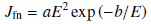
Hereby a and b are material specific constants which reflect the material's work function and the surface's shape, E is the absolute value of the electric field. This kind of emission typically starts to occur in the presence of very high electric fields in the range of 10e9 - 10e10 V/m. The relation between the electric field and emitted current density is shown in the following diagram:
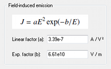
The following section in the ”Define Field-Induced Emission” dialog box offers the possibility to set the values of the field-induced emission parameters:
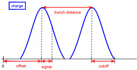
The Gauss emission model consists in a pulsed particle emission. The particles are emitted with an initial velocity that is determined by the kinetic settings. The pulses are Gaussian in the sense that the emitted charge of each pulse is a Gaussian curve as a function of time. The user can specify various parameters of the Gaussian pulses (or bunches), such as the total charge of each pulse, the pulse width or the time interval between two successive pulses. In the absence of fields, and when the particles have the same initial velocity, the pulses that are defined to be Gaussian in time have a Gaussian shape in space too. Then the aforementioned parameters of the Gaussian pulse can be also defined in space. It should be noted that the emission is still Gaussian in time, as the spatial parameters are transformed in their equivalent temporal counterparts, using the user-specified kinetic settings, i.e. the initial velocity. The possibility to define a Gaussian pulse spatially is convenient in cases in which the Gaussian pulse parameters are know in space, e.g. in cases of beams in particle accelerators . The user can select between setting the Gaussian pulse parameters in time or space by checking the boxes "Time" or "Length" respectively.
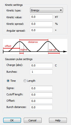
The charge is uniformly distributed over the emission surface. A charge with a Gaussian charge distribution vs. time leaves a particle area source:
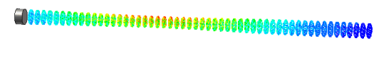
At each time-step new particles with a fraction of the total bunch charge are created and emitted from the surface.
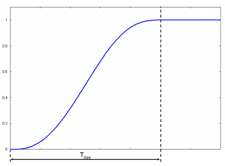
Within the "Define DC Emission Model" dialog box the kinetic and current settings for the fixed emitted particle beam can be entered. To avoid high frequency problems which would be caused by a step function, a finite rise time for the current must be defined.
The following plot shows the rise of the current within the rise time Trise. After the time Trise the source emits the fixed current that is specified within the "Current Settings" group.
For circular sources, the oblique emission feature is available as a part of the DC emission model. By clicking on the More>> button, the user can edit the oblique emission settings.
Within the field emission dialog box, the kinetic settings and parameters for this emission model can be entered.
The field emission model for the particle in cell solver is based on the Fowler Nordheim equation. Here a and b are positive material-specific constants which depend on the material work function and on the surface shape, E is the absolute value of the electric field dependent from the time.
This kind of emission typically starts to occur in the presence of very high electric fields, typically in the range of 109 - 1010 V/m. The dependence of the emitted current density on the electric field is shown in the following diagram:
In each time step, the emitted particles decrease the electric field in the vicinity of the cathode. Thus, if the charge of the emitted particles is too strong, the emission process will stop.
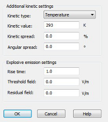
The explosive emission is an electric field-dependent process. Emission starts when the electric field strength close to the cathode is greater than a user-specified threshold. This condition is verified for every particle once: if the emission process starts, this field threshold has no effect of the particle again.
By default, the charge of the emitted particles is calculated in such a way that the electric field vanishes in the region near the cathode. Typically, due to the high electric field thresholds, these calculations lead to such a rapid increase of the emitted charge that instabilities occur because of the high frequency content. To avoid this non-physical behavior, the calculated emitted charge is multiplied with the following factor, which increases smoothly as a function of time:
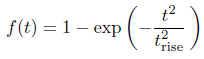
The rise time can be adjusted by the user to avoid instabilities or non-physical behavior. The default condition that the electric field close to the cathode vanishes can be modified:a finite field can remain in the cathode region and the user can specify a value for the so-called residual field. The parameters that have been previously described, as wells as the kinetic settings, can be entered in the explosive emission dialog box.
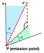
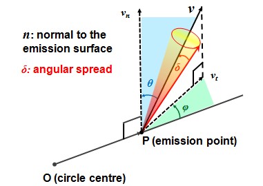
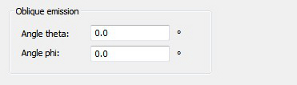
For circular particle sources, particle emission can be oblique with respect to the surface of the source, i.e. the particles can be emitted with a velocity that forms a finite angle theta with the source surface normal. The emission velocity v has then two components: the component vn, that is parallel to the surface normal, and the component vt, that is perpendicular to the surface normal and lies in the source plane. The component vt is fixed by specifying the angle phi with respect to the straight line defined by the center of the circular source O and the emission point P. When the angle theta is zero, vt is zero, so changing the setting for angle phi cannot affect the particle emission properties.
When a finite angle spread delta is specified in the kinetic settings section, the emission vector is randomly distributed inside a conic region. The axis of this conic region is defined by the fixed vector v and the maximum angle between the generatrix (cone's lateral surface) and the axis is given by the angle spread.
The oblique emission feature is available in the Fixed emission model in the Tracking solver and in the DC emission model in the PIC solver.
See also
Particle Area Source, Particle Point Source, Particle Circle Source, Secondary Electron Emission
TRK - Fixed Emission, TRK - Space Charge Limited Emission, TRK - Thermionic Emission, TRK - Field-Induced Emission
PIC Gauss Emission Properties, PIC DC Emission Properties, PIC Field Emission Properties, PIC Explosive Emission