Which Solver To Use

CST PARTICLE STUDIO features six different field solvers the electrostatic, the magnetostatic, the eigenmode solver, the particle tracking solver, the particle in cell solver (PIC) and the wakefield solver.

Since an iterative method is used, all field solvers have in common that a stop accuracy has to be supplied. The stop accuracy is important for further post processing, since it limits the accuracy of secondary results. On the other hand it is a rule of thumb that more accuracy needs more solver time.

Eigenmode Solver

In cases of strongly resonant loss-free structures, where the fields (the modes) are to be calculated, the eigenmode solver is very efficient. This kind of analysis is often useful for determining the poles of a highly resonant filter structure. But of course there are different applications for the eigenmode solver: with periodic boundaries and a non-zero phase shift for instance, the eigenmodes are traveling waves. The eigenmode solver directly calculates the first N frequencies for which fields may exist in the structure, and the corresponding field patterns. In case of the JDM eigenmode solver and the eigenmode solver with tetrahedral mesh a frequency target could be chosen such that the eigenmodes are calculated from the frequency target in ascending order. The eigenmode solver can not be used with open boundaries or discrete ports. Electrically lossy materials can be handled by the lossy JDM eigenmode solver method if the assumption of a complex frequency independent permittivity is valid.

Magnetostatic Solver

The magnetostatic solver can be used for static magnetic problems. Available sources are current paths, current coils, permanent magnets and homogeneous magnetic source fields as well as the current density field previously calculated by the stationary current solver. To use the J-static current density field as magnetostatic source, select SolveStationary Current Field... and enter a Factor larger than 0. The main task for the solver is to calculate the magnetic field strength and the flux density. These results appear automatically in the navigation tree after the solver run.

Nonlinear Materials

The magnetostatic solver also features nonlinear materials. When these are defined the permeability distribution inside the material has to be computed. Thus mostly more than one linear solver run has to performed and so the permeability distribution calculated. As a result the permeability distribution is also stored and can be accessed in the navigation tree.

Open boundaries

Open boundary conditions are useful for problems that do not interact with the space outside the calculation domain. Thus it simulates the structure in open space.

See Magnetostatic Solver Overview.

Electrostatic Solver

The electrostatic solver can be used for static electric problems. Available sources are fixed and floating potentials, boundary potentials, charges on PEC solids and homogeneous volume and surface charges. The main task for the solver is to calculate the electric field strength and the flux density. These results appear automatically in the navigation tree after the solver run.

Open boundaries

Similar to magnetostatics, the electrostatic solver features open boundary conditions. These help to reduce the number of mesh nodes, when problems in free space are simulated.

See Electrostatic Solver Overview.

Gun Solver & Particle Tracking

The particle tracking solver can be used to compute trajectories of charged particles within electrostatic, magnetostatic or eigenmode fields. The implemented gun-iteration enables the computation of a self-consistent electrostatic field which considers the reaction of the particle movement to the electrostatic potential distribution. As particle sources arbitrary shaped surfaces of solids can be defined. These surfaces emit particles considering a predefined emission model. The main task for the solver is to calculate the particle trajectories, the self-consistent electrostatic field, the space charge distribution and the particles' current. These results appear automatically in the navigation tree after the solver run.

Multiple Particle Source definitions

The particle tracking solver offers the tracking of different particle types from different sources independently. Thus the simulation of multibeam guns or the parallel simulation of particle beams is possible.

See Tracking Solver Overview.

PIC Solver

The PIC solver can simulate charged particles in self-consistent electromagnetic fields. Moreover static or analytic field distributions can be added to the PIC simulation. Charged particles can be emitted from arbitray surfaces or single points. Moreover electromagnetic fields can be stimulated by previously defined ports.

See PIC Solver Overview.

Wakefield Solver

The wakefield solver can be used to compute wakepotentials of charged particle bunches. Therefore the electromagnet fields are calculated with a time domain solver and integrated in a postprocessing step. Wakepotentials deliver important information for the design of particle- accelerators. See Wakefield Solver Overview.

Thermal Stationary Solver

The thermal stationary solver can be used to simulate temperature distribution problems.

For detailed information please refer to the Thermal Stationary Solver Overview page.

Thermal Transient Solver

The thermal transient solver can be used to simulate time-dependent temperature distribution problems.

For detailed information please refer to the Thermal Solver Overview page.

General Hints

Please consider the following general hints on how to increase the performance of your simulation runs.

Always make use of geometric symmetry planes.
Avoid an unnecessarily large calculation domain size.
Consider using the distributed computing options.

Result Data Caching

For further processing of single runs within a multi-run (e.g. Parameter Sweep, Optimization) all models and results can be stored in subfolders on the hard disk when checking the ”Store results in data cache” option. This might be very helpful for own macros or just to check a single run.

Adaptive Mesh Refinement

For all solvers an adaptive mesh refinement can be activated. Therefore the mesh will be refined until the change of the results from one pass to the other deviate less than the given limit in percent. This option produces very good simulation results without the need for manual mesh tuning.

Capacitance / Inductance / Conductance Matrix

The calculation of the capacitance, inductance or conductance matrix is another feature available for electrostatics, magnetostatics or for the stationary current solver, respectively.

For electrostatics the capacitance matrix C for all n source definitions can be calculated.

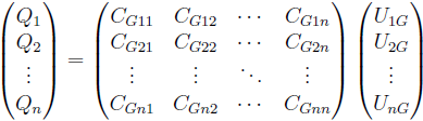
Here, Q and V denote the vectors of the conductor charges and potentials, respectively.

In order to calculate the complete matrix n solver runs have to be performed.

The inductance matrix L is the corresponding equivalent for magnetostatics.

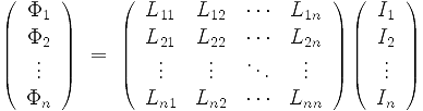
Here, Φ and I denote the vectors of the coil and path fluxes and currents, respectively.

In the special case, where at least on coil is defined, the number of solver runs equals 0.5*n*(n+1). Otherwise n solver runs are sufficient in order to calculate the complete inductance matrix.

Please note that if nonlinear materials are defined the inductance is not independent of the source current. Therefore no meaningful inductance matrix can be calculated.