
A step-by-step description of how to construct an electrostatic model and set up the simulation is available in the Tutorials under Example Overview.
Solver specific sources
The following sources are available:
|
• Potentials on conductors (fixed or floating) |
|
|
• Boundary potentials (fixed or floating) |
|
|
| |
|
• Charges on PEC solids |
|
The electrostatic solver features open boundary conditions. They help to reduce the number of mesh nodes, when problems in free space are simulated.
A capacitance matrix can be computed automatically by the electrostatics solver.
The potential definitions on PEC objects are used to define regions which are considered in the capacitance matrix. All PEC regions which do not carry a potential definition are considered as ground conductor.
Please note: Charge definitions are not taken into account for the definition of the capacitance matrix.
Please note that symmetries can have an influence on the capacitance values. In particular, if a symmetry plane is defined, then each shape which is not cut by this plane is considered a union of itself with its counterpart on the other side of the symmetry plane. This means that potential sources on such shapes cannot be excited separately. If you combine symmetries with a capacitance calculation, please check your results carefully.
For a capacitance matrix with n lines and columns, n solver runs are required.
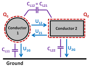
Two different types of capacitances are computed and available in the result tree
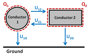
A simple
setup with two conductors defined by a potential definition and an additional
ground conductor.
The capacitances are describing the relation between voltages U and charges
Q.
Grounded Capacitance Matrix
The grounded capacitance matrix describes the relation between the voltages to ground and the charges on the conductors. For the setup above the matrix equation would look as follows:
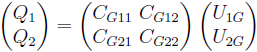
If the ground conductor has a potential of 0V, the voltage is equal to the potential on the conductors.
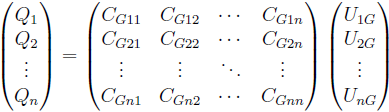
For a system with n conductors the grounded capacitance matrix looks as follows:
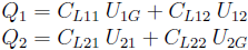
Lumped Capacitance Matrix
Many applications require the knowledge of capacitance values which are based on voltages between conductors (instead of voltages to ground). They are often referred as lumped capacitances. For the setup in the picture above, the lumped capacitance matrix can be described by the following equations:
With lumped capacitances the coupling between conductors can be easily illustrated:
A system described by lumped capacitances can be easily transferred to a circuit simulator.
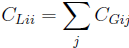
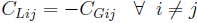
The lumped capacitance matrix can be easily obtained from the grounded values:
Both matrices are always symmetric.
Open boundaries
The electrostatic solver features open boundary conditions. These help to reduce the number of mesh nodes, when problems in free space are simulated.
It is possible to choose between a charge-free open boundary or a fixed potential boundary at infinity.
Mesh Type
The electrostatic solver supports tetrahedral as well as hexahedral meshes.
General Hints
Please consider the following general hints on how to increase the performance of your simulation runs.
Always make use of geometric symmetry planes.
Avoid an unnecessarily large calculation domain size (e.g. use open boundary conditions is necessary).
Result Data Caching
For further processing of single runs within a multi-run (e.g. Parameter Sweep, Optimization) all models and results can be stored in sub-folders on the hard disk when checking the ”Store results in data cache” option. This might be very helpful for own macros or just to check a single run.
Adaptive Mesh Refinement
For the solver an adaptive mesh refinement can be activated. Therefore the mesh will be refined until the change of the results from one pass to the other deviate less than the given limit in percent. This option produces very good simulation results without the need for manual mesh tuning.
See also
General Solver Overview, Electrostatic Solver Parameters, Boundary Conditions-Boundaries, Electrostatic Sources, Define Potential, Boundary Conditions-Boundary Potentials, Define Volume or Surface Charges, Define Charge on PEC solid