Boundary Conditions - Boundaries

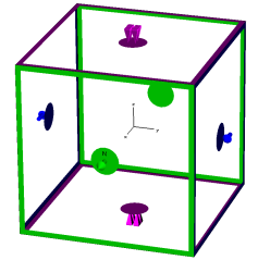
Due to the fact that a computer is only capable of calculating problems that have finite expansion, you need to specify the boundary conditions. This can be done within this dialog box.

When you enter the boundaries property sheet, the modeled structure is displayed with a surrounding bounding box colored with regard to the boundary condition at each boundary. The picture on the right shows an example of such a bounding box.

The assignment of the colors to the boundary conditions is listed together with the description of the different boundary conditions below.

Electric: Operates like a perfect electric conductor, where the tangential components of electric fields and the normal components of magnetic fluxes are zero. This means that electric fields are normal to the boundary and magnetic fluxes are parallel to the boundary. For all magnetostatic or magnetoquasistatic applications electric boundary conditions correspond to tangential boundary conditions. For all electrostatic or electroquasistatic applications they correspond to normal boundary conditions. This boundary condition type is available for all EMS solvers.

Magnetic: Operates like a perfect magnetic conductor, where the tangential components of magnetic fluxes and the normal components of electric fields are zero. This means that electric fields are parallel to the boundary and magnetic fluxes are normal to the boundary. For all magnetostatic or magnetoquasistatic applications magnetic boundary conditions correspond to normal boundary conditions. For all electrostatic or electroquasistatic applications they correspond to tangential boundary conditions. This boundary condition type is available for all EMS solvers.

Open:

Electrostatic, magnetostatic and thermal solver
Operates like free space.

PIC solver (PML)
Operates like free space: Waves can pass this boundary with minimal reflections. Additionally, charged particles can be absorbed by the PML. Only available for PIC on CPU.

Wakefield solver (PML)
Operates like free space: Waves can pass this boundary with minimal reflections.

Open (add space):

PIC and wakefield solver
Same as Open (PML), but adds some extra space (vacuum) between the bounding box of your model and the open boundaries.

Open (add space lf):

Electrostatic, magnetostatic  and thermal solver
Similar to the open boundary condition, with some extra space added between structure and applied boundary condition.

Normal: Forces the tangential components of the electric, magnetic or current field (depending on your application) to be zero at the boundary. This means that the corresponding field has only normal components at the boundary. For all magnetostatic or magnetoquasistatic applications normal boundary conditions correspond to magnetic boundary conditions. For all electrostatic or electroquasistatic applications they correspond to electric boundary conditions. This boundary condition type is available for the electrostatic, magnetostatic stationary current and thermal solver.

Tangential: Forces the normal components of the electric, magnetic or current field (depending on your application) to be zero at the boundary.  For all magnetostatic or magnetoquasistatic applications tangential boundary conditions correspond to electric boundary conditions. For all electrostatic or electroquasistatic applications they correspond to magnetic boundary conditions. This boundary condition type  is available for the electrostatic, magnetostatic stationary current and thermal solver.

Magnetic boundary

Electric boundary