PIC Solver Overview

The Particle In Cell solver (PIC) calculates the development of fields and particles through time at discrete time samples. Fields are computed at discrete locations whereas particles are tracked in continuous phase space.

The fields are calculated step by step through time by the ”Leap Frog” updating scheme. It is proven that this method remains stable if the step width for the integration does not overcome a known limit. This value of the maximum usable time step is directly related to the minimum mesh step width used in the discretization of the structure. Therefore, the denser the chosen grid, the smaller the usable time step width. This stability condition does not apply to the particle update scheme.

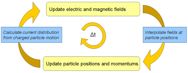
Since the particle in cell scheme is a self-consistent simulation method for particle tracking, it is necessary to interpolate fields for the particle motion and particle currents for the field computation. Both interpolation schemes are linear.

How to start the solver

Before you start the solver you should make all necessary settings. The PIC solver can be started from the PIC Solver Parameters dialog box. The solver can only be started if at least one particle source has been defined. At solver start all previously calculated results will be deleted. It is advisable to define an particle position monitor additionally.

Solver logfile

After the solver has finished you can view the logfile by clicking Results Solver Logfile in the main menu. The logfile contains information about solver settings, mesh summary, solver results and solver statistics.

Results

In the navigation tree the field calculation results are added under "2D / 3DResults".

The particle position monitor plots are accessible via "2D / 3DResults / Particles".

Features

Different emission models (e.g. Gauss, DC and Field Emission) can be used to emit particles.
Secondary electron emission based on the Furman emission model.
Static and predefined electric and magnetic fields.
Calculation of the time averaged power to couple the PIC solver to the thermal solver.
Sheets can be chosen to be transparent for particles.
Particle position monitors to record 3D trajectory data.
PIC 2D monitors to get detailed particle data information on a 2D plane in the 3D space.
Phase space monitors to get e.g. a 2D plot energy vs. z.
At PEC bodies non-physical space charge due to current mapping can be avoided. This features decreases the solver performance slightly.
Particle interfaces can be used to export particles (e.g. from a gun simulation) from the tracking solver into the PIC solver. Within an bounding box around the interface emitted particles are tracked only by static forces.

Simulation Acceleration

CPU parallelization

The PIC solver is parallelized with OpenMP. The number of threads, that the solver is allowed to use, can be defined by the user.

GPU support

The PIC solver supports single GPU calculations. A minimum compute capability of 2.0 (e.g. Tesla-Fermi) is required to run a PIC GPU simulation. Read the GPU documentation for further details.

Nearly all CPU features are available for the GPU solver, but five features are (currently) missing: PIC 2D Monitors / Secondary Electron Emission / Particle Interfaces / Sheet Transparency for Particles / Modulation of External Fields.

Distributed Computing

The Distributed Computing system allows the distribution of independent simulation runs over several computers within a network.