
The magnetostatic solver can be used for static magnetic problems. The main task for the solver is to calculate the magnetic field strength H and the flux density B. Furthermore, the energy and the source current density are displayed. In case coils were defined also flux linkages are computed. These results appear automatically in the navigation tree after the solver run.
Solver specific sources
The following solver specific sources are available:
|
| |
|
| |
|
| |
|
| |
|
|
Stationary current fields
Additionally, a stationary current field in conductive regions can be used to drive the magnetostatic problem. To run the stationary current solver before the magnetostatic calculation, just check the "Precompute stationary current field" check-box in the solver dialog. It is important that the stationary problem with its sources and boundary conditions is well defined, otherwise the whole simulation will be aborted with an error message.
Nonlinear Materials
The magnetostatic solver also features nonlinear materials. When these are defined the permeability distribution inside the material has to be computed. Thus mostly more than one linear solver run has to performed and so the permeability distribution calculated. As a result the permeability distribution is also stored and can be accessed in the navigation tree.
PEC Materials
In a magnetostatic simulation, PEC material is considered like an internal electric boundary, i.e., there are only tangential components of the H-Field at the PEC surfaces. This behaviour can be changed for particle tracking simulations (in combination with hexahedral meshes).
The calculation of the apparent inductance matrix is another feature available for magnetostatics.
Each coil segment and current coil definition increases the dimension n of the apparent inductance matrix L by one. If coils are defined the calculation of the apparent inductance matrix requires n additional solver runs. When only one current source has been defined, only one single run is necessary to compute the self inductance. The apparent inductance matrix relates the flux linkages to the currents by:
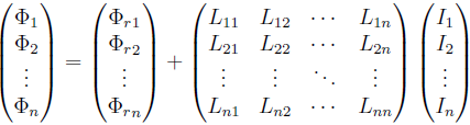
Here, Φ and I denote the vectors of the coil flux linkages and currents, respectively, and Φr denotes the vector of magnetic flux originating from current independent sources e.g. permanent magnets.
Please note, that if nonlinear materials are defined the inductance depends on the source current.
Open boundaries
Open boundary conditions are useful for problems that do not interact with the space outside the calculation domain. Thus it simulates the structure in open space.
Mesh Type
The magnetostatic solver supports tetrahedral as well as hexahedral meshes.
General Hints
Please consider the following general hints on how to increase the performance of your simulation runs.
Always make use of geometric symmetry planes.
Avoid an unnecessarily large calculation domain size.
Result Data Caching
For further processing of single runs within a multi-run (e.g. Parameter Sweep, Optimization) all models and results can be stored in subfolders on the hard disk when checking the ”Store results in data cache” option. This might be very helpful for own macros or just to check a single run.
Adaptive Mesh Refinement
For the solver an adaptive mesh refinement can be activated. Therefore the mesh will be refined until the change of the results from one pass to the other deviate less than the given limit in percent. This option produces very good simulation results without the need for manual mesh tuning.
See also
Solver Overview, Magnetostatic Solver Parameters, Boundary Conditions-Boundaries, Magnetostatic Sources, Define Current Path, Define Current Coil, Define Coil Segment, Define Permanent Magnet, Define Magnetic Source Field, Stationary Current Solver, Flux Linkage