Wakefield Solver Overview

The wakefield solver calculates the so called wake-potentials for a given structure from electromagnetic fields. Wakefield problems are driven by a bunch of charged particles, which is passing the observed structure parallel to a main coordinate axis. These particles cause electromagnetic fields, which are calculated with a time domain solver.

The wake potential W(s) can be used to describe the change of momentum on a test charge q2, which is at a distance s behind the excitation bunch q1:

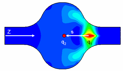
The wake potential (including longitudinal and transversal components) can be derived from the electromagnetic fields by evaluating the following integral:

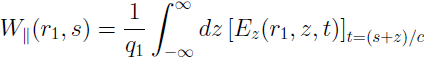
The computation of the longitudinal component even simplifies to an integration of Ez, since the magnetic fields do not contribute to this component:

If the tangential components of the electric field vanishes on the integration boundaries, the so called Panovsky-Wenzel theorem can be used to compute the transverse wake components directly from the longitudinal one (see also [1]):

Therefore it is necessary to compute the electromagnetic fields step by step through time by the so called ”Leap Frog” updating scheme. It is proven, that this method remains stable if the step width for the integration does not exceed a known limit. This value of the maximum usable time step is directly related to the minimum mesh step width used in the discretization of the structure. So, the denser the chosen grid, the smaller the usable time step width.

In a second step the wake potentials can be calculated by integrating the electromagnetic fields along the z-axis (direct integration scheme). Another calculation method integrates the electromagnetic fields only at discontinuities. This can be more accurate, but has higher requirements on the model and the beam (see also: Wakefield Calculation Settings).

Further information about wake potentials and the relation between longitudinal and transversal components can be found in [1].

Note if beams are significantly slower than the speed of light, the indirect wake computation methods are not available. Moreover the wake potential depends not only on the geometry of discontinuities but also on the length of the simulated beam tubes. Results must be interpreted with special care in this case.

How to start the solver

Before you start the solver you should make all necessary settings. The wakefield solver can be started from the Wakefield Solver Parameters dialog box. The solver can only be started if at least one particle beam source has been defined. At solver start all previously calculated results will be deleted.

Solver logfile

After the solver has finished you can view the logfile by clicking Post Processing: Manage Results Logfile . The logfile contains information about solver settings, mesh summary, solver results and solver statistics.

Results

In the navigation tree the calculation results are added under "1D Results\Partilce Beams\<beamname>" for each particle beam excitation. The most important entries are listed below:

Current

Shows the beam current at the entry point versus time.

Charge distribution (time / distance / spectrum)

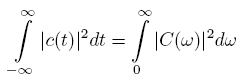
Shows the charge distribution versus time or distance from the barycenter of charge. The single sided charge distribution spectrum (amplitude) is the fourier transformation of the time signal.

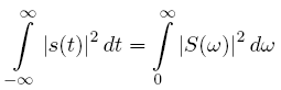
Note: The fourier transform is normed such that the unitarity is given or Parseval's identity is fulfilled:

Wake Potential

The wake potentials for every component are added together with a normed reference pulse in this folder. The height of the reference pulse is always normed to the maximum of all wake potential functions, its purpose is to indicate the location of the reference charge q1 only.

Wake Loss Factor

The wake loss factor (k) for the longitudinal wake component is calculated by:

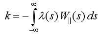
were lambda(s) describes the normed charge distribution function over s (to obtain the charge distribution one has to multiply this function by q1). It is given in [V / pC].

Kick Factor

If the wake integration line has an offset to the beam-line a transversal Kick factor is calculated automatically by:

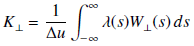
This computation is very similar to the calculation of Wake Loss Factor, but in addition the integral is divided by the distance of the wake integration line to the beam line (du).

It is given in the unit [V / pC / <Userdefined dimension unit>]. This means if the structure was defined in mm the kick-factor is given in V / pC / mm.

Wake Impedance

The longitudinal wake impedance is computed by the fourier-transformation of the longitudinal component of the wake potential, which is divided by the fourier-transformed charge distribution function lambda(s).

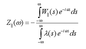
The transversal wake impedance is given by:

Note: The scaling factor of -i for the transverse impedance is commonly used in literature (see also [1]).

A single sided DFT with 1000 frequency samples is used for the numerical fourier transformation:

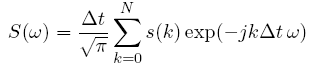
with:

dt: time sampling width.

N: number of time samples

w: angular frequency (1000 samples)

This fourier transform preserves Parsevals identity with omega:

References

[1] T.Weiland and R. Wanzenberg, Wake fields and impedances, Proc. of the CAT - CERN Accelerator School (CCAS), pp.140-180, 1993