Wakefield Calculation Settings

Simulation: Sources and LoadsParticle BeamWakefields

Wake integration method

Select between the direct or two indirect integration methods to compute the wake potential. A good overview for the different indirect integration methods can be found here in [1].

Direct

The direct method is the most general method but also less accurate than the two indirect methods. It is used if the particle beam is not ultrarelativistic, or if an indirect method is not applicable.

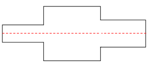
The wake potential is computed by an integration along an axis parallel to the beam axis.

Indirect testbeams

This is the most accurate integration method. It can be used if the beam has an ultrarelativistic velocity and the beam tubes cross section at the entry boundary equals the cross section at the exit boundary. In addition the structure must not be concave which means basically that the cross section of the part between the beam tubes must be larger than the tubes cross section. As a consequence a collimator can not be treated with this integration method in general. The method is described more detailed in [2].

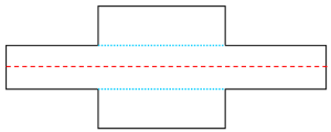
The wake potential is computed via recording the longitudinal field values on the extruded shell of the beam tube in the discontinuous region (blue lines).

Indirect interfaces

If the cross section of the beam tube varies at the entry and the exit boundary, one can choose this method for ultrarelativistic beams. The method is described more detailed in [3].

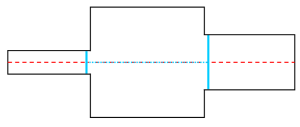
The wake integration in the discontinuous region is done directly on an axis parallel to the beam (dotted blue line). For the tube regions the wake potential share is considered by a computation on the interface areas (thick blue lines).

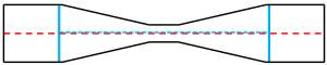
Concave structures can not be treated with the Indirect testbeams method, but with the Indirect Interfaces.

If the solver recognizes than an indirect integration scheme can not be applied, the direct method is used and a warning will be printed.

Integration path shift X/Y/Z

Determine if the wakefields have to be computed on an axis which is shifted transversal to the particle beams axis. Only two edit boxes are active, since a longitudinal axis shift is not useful.

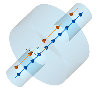
The particle beam axis is visualized by the blue line, while the orange line shows where the wakefields will be computed. In this case the particle beam moves along the z-axis and the wake integration path is shifted in x-direction.

Wake Impedance Spectrum

For the wake impedance calculation a cos² filtering is available in order to generate a smooth spectrum for highly resonant structures. The filter function is multiplied with the wake function before the fourier analysis is performed.

Note: Wake impedance spectra can also be calculated after a simulation is finished. See also: Wakefield Postprocessor.

Apply cos² filtering

Check this box to switch on the filtering.

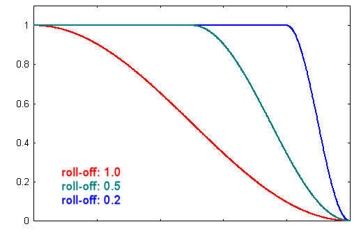
Roll off factor

The roll-off factor can be chosen between 0 and 1. A high value means that the filter is relative smooth, a small value defines a steep filter ramp.

Performs your settings and leaves the dialog box.

Cancel

Closes this dialog box without performing any further action.

Help

Shows this help text.

Wakefield Calculation Settings

Simulation: Sources and LoadsParticle BeamWakefields

Simulation: Sources and LoadsParticle BeamWakefields

References:

[1] Igor Zagorodnov, Indirect methods for wake potential integration, Physical Review Special Topics - Accelerators and Beams 9, 102002 (2006)
[2] T. Weiland and R. Wanzenberg, Wake Fields and Impedances, CCAS-CAT-CERN Accelerator School, Indore, November 1993, p. 140.
[3] H. Henke and W. Bruns, Calculation of Wake Potentials in General 3D Structures, Proceedings of EPAC 2006, Edinburgh, Scotland (WEPCH110, 2006)