Modeler View

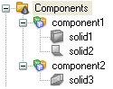
Components: In the navigation tree all components are displayed together with their associated solids. In order to distinguish single faces (solid2), from normal solids (solid1) and from mixed bodies (solid3), which include face and solid parts, all three types are indicated by different icons.

If a specific component is selected all its solids are visualized while the others are displayed transparently. If a single specific shape is selected, only this shape is visualized differently.

You can easily copy solids by means of the Copy and Paste Solids feature.

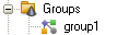
Groups: This is a convenient way to group objects (i.e. solids and wires) together. You can define 2 different kinds of groups i.e. Normal group   and Mesh group .

A normal group allows you to hide or show multiple objects at once. A mesh group offers the functionality of a normal group and in addition allows you  to define local mesh properties. Objects which are part of a mesh group inherits the local mesh properties from it. If there are multiple objects under a mesh group, they share the same local mesh properties.

An object cannot coexist in multiple groups of the same type i.e. It can be a part of a mesh group and a normal group at the same time, but cannot be a part of two different mesh groups or normal groups at the same time.

'Excluded from Simulation' and 'Excluded from Bounding Box' are two utility groups which are available by default. You can add objects to these groups, to exclude them from simulation or the bounding box.

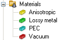
Materials: If a specific material is selected all its solids are visualized while the others are displayed transparently.

Faces: In the navigation tree all faces are listed as green surfaces, in the main plot window they are also displayed in green. However, their color can be changed in the Colors View Options dialog.

Curves: In the navigation tree all curves as well as their associated curve items (lines, circles, ellipses, rectangles, polygons, splines, 3D polygons)0 are listed. In the main plot window they are displayed in blue, however, this color can be changed in the Colors View Options dialog.

Wires: In the navigation tree all wires are listed as blue curves, in the main plot window they are highlighted in orange. However, their color can be changed in the Colors View Options dialog.

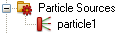
Particle Sources: All particle sources are listed under this folder. When the particle source folder is selected, all particle emitting surfaces are highlighted and coloured according to their specific q/m ratio of the corresponding particle types.  If all particles sources are defined on PEC surfaces, the non PEC solids are displayed transparent. If a single source definition is selected all other particle sources are not colored

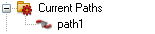
Current Paths: All current paths are usually shown in blue.

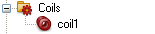
Coils: All coils are shown in coppery and the direction of the current is visualized with gray arrows.

Potentials: When the potentials folder is selected all potential definitions are shown, colored with respect to the potential value and the chosen color ramp. All other non PEC solids are displayed transparent. If a single potential definition is selected all other potentials are not colored

Charges: The charge folder contains all charge definitions. If it is selected, all charges are visualized. Similar to the potentials, the faces of the charge definition is colored in consideration of the charge value and the chosen color ramp. When a specific charge is selected, all other charges are not colored.

Permanent Magnets: All permanent magnet definitions are accessible under the Permanent Magnets folder.  If the permanent magnet folder is selected, all permanent magnet definitions are displayed. The color of the definition represents the absolute value of the magnetization in reference to the color ramp. For a single permanent magnet selection all other definitions will be neglected for the visualization.

Excitation Signals: Excitation Signals describe the excitation function used for the transient stimulation of the defined sourcesport signals. Multiple signals , can be defined either manually or loaded from the Excitation Signal Library. A so called "Reference Signal" (indicated by the icon) is used as default stimulation in a normal transient solver run for stimulating the port modes, but performing a simulation with selected port modes and activated simultaneous excitation setting allows the stimulation of different ports with different excitation signals in one solver run.

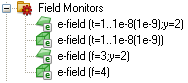
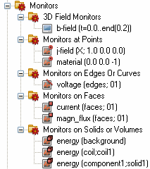
Field Monitors: All 2D monitors are visualized as a plane positioned at the specified location in the same color as their symbol in the navigation tree. Corresponding to this the 3D monitors are plotted as a colored wire frame box. This applies for the frequency monitors as well as for the time monitors.

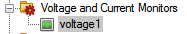
Voltage Monitors: These monitors are visualized in the main plot window as a line or curve with a cone in the middle, all highlighted in dark green. However, this color can be changed in the Colors View Options dialog.

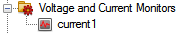
Current Monitors: These monitors are visualized in the main plot window as a line or curve with a cone in the middle, all highlighted in dark green. However, this color can be changed in the Colors View Options dialog.

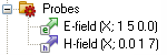
Probes: The probes are shown as arrows with a point at the actual probe position in the same color as their symbol in the navigation tree.

3D Field Monitors are used for the transient/time-domain solvers to compute a field in a given time frame. Each defined 3D Field Monitor will produce a vector field in the 2D/3D Results folder which can be animated over time..

Monitors at Points, Monitors on Edges or Curves, Monitors on Faces and Monitors on Solids or Volumes are indicated by a point, a line, a rectangle or a brick in the upper right corner of the icon, respectively. These monitors allow to observe certain physical quantities on different geometric entity and yield a real-valued scalar function (quantity vs. time) in the 1D Results folder.