
The stationary current solver can be used to simulate stationary current fields. The main task for the solver is to calculate the electric field strength E and the conduction current density. These results appear automatically in the navigation tree after the solver run.
Solver specific sources
The following sources are available:
|
| |
|
| |
|
| |
|
| |
|
| |
|
|
Conductance Matrix
The calculation of the conductance matrix is another feature available of the stationary current solver.
Each current port or defined potential increases the dimension n of the conductance matrix G by one and the calculation requires n solver runs.
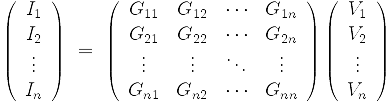
Here, I and V denote the vectors of the currents and the potentials, respectively.
Boundary conditions
Normal or electric boundary conditions impose normal components of the current field (or electric field) at the corresponding boundaries.
Tangential or magnetic boundary conditions force the normal components of the stationary current or electric field to be zero at the corresponding boundaries.
Open boundary conditions are currently not supported by the stationary current solver.
A source definition at a boundary overwrites the boundary condition at the position of the source. For example, a current port will impose a normal current field no matter where it is positioned.
Please note that in a stationary current simulation the computational domain is restricted to the union of conductive shapes (including solids or wires with PEC or conductive materials, current wires and lumped elements). Hence, the boundary conditions are restricted to the boundary of the computational domain. This means, in particular, that settings for boundary parts which are not adjacent to any conductive region are ignored by the stationary current solver.
Lumped Network Elements
Use lumped elements to include electrical component into the simulation. Only resistances are supported by the stationary current solver.
Supported Material Properties
The stationary current solver delivers the distribution
of scalar potentials within the regions with non-zero electric conductivity
 . The
following material properties are supported:
. The
following material properties are supported:
Anisotropy: the diagonal elements of electric conductivity tensor can be defined along with the local solid coordinate system.
Temperature dependency: electric conductivity can depend on temperature (feature currently supported only by the tetrahedral solver). The temperature distribution can be imported from a hexahedral or tetrahedral stationary thermal solution. The shape of temperature dependency can be defined in the Temperature Dependent Materials dialog.
Nonlinearity: electric conductivity can also depend on the electric field (feature currently supported only by the tetrahedral solver). In this case the nonlinear solution is started. The nonlinearity can be defined as a dependency of electric field E on electric current J in the Nonlinear Electric Conductivity dialog.
Please note that these features cannot currently be combined for the same material. For more information please refer to Material Overview (LF).
Mesh Type
The stationary current solver supports tetrahedral as well as hexahedral meshes.
General Hints
Please consider the following general hints on how to increase the performance of your simulation runs.
Always make use of geometric symmetry planes.
Avoid an unnecessarily large calculation domain size.
Result Data Caching
For further processing of single runs within a multi-run (e.g. Parameter Sweep, Optimization) all models and results can be stored in subfolders on the hard disk when checking the ”Store results in data cache” option. This might be very helpful for own macros or just to check a single run.
Adaptive Mesh Refinement
For the solver an adaptive mesh refinement can be activated. Therefore the mesh will be refined until the change of the results from one pass to the other deviate less than the given limit in percent. This option produces very good simulation results without the need for manual mesh tuning.
Solver Results
The following 3D distributions are generated by the stationary currents solver:
Scalar potential within conductive materials.
Electric field strength E.
Stationary current density J.
If materials with temperature-dependent electric conductivity are present, the distribution of imported temperature in K within these materials is visualized (only for tetrahedral-based solver).
If materials
with temperature-dependent or nonlinear electric conductivity are present,
the distribution of electric conductivity within these materials is visualized (only
for tetrahedral-based solver).
See also
General Solver Overview, Stationary Current Solver Parameters, Boundary Conditions-Boundaries, Stationary Current Sources, Boundary Conditions-Boundary Potentials, Define Potentials, Define Current Path, Define Coil Segment, Define Current Port, Lumped Elements