Eigenmode Solver Overview
The eigenmode solver is used to calculate the frequencies and the corresponding
electromagnetic field patterns (eigenmodes), where no excitation is applied.
Loss free structures are supported (losses are available with the JDM
method and hexahedral mesh, or by means of the perturbation method), without
open boundaries.
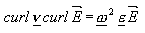
The eigenmodes and their frequencies are the solutions of the eigenvalue
equation
with the complex permittivity and reluctivity
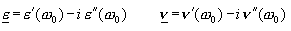
respectively. The complex permittivity (reluctivity) is evaluated at
a given material
evaluation frequency. The complex angular frequency is related to
the real angular frequency and the Q-factor by
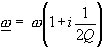 . .
Which eigenmode solver method to use
With hexahedral mesh, two eigenmode
solver methods are available and will be shortly described in the following:
The Advanced Krylov Subspace method (AKS), and the Jacobi-Davidson method
(JDM), which is capable to also solve lossy structures.
Normally, only a finite number of the lowest eigenmodes are needed.
Therefore, the AKS solver uses a special filter polynomial to suppress
the unwanted higher modes. The solver works in frequency domain using
an iterative subspace method.
The AKS method depends on an estimation of the eigenvalue of the highest
mode under consideration. This estimation is chosen automatically during
an iterative estimation refinement process. If many of these passes are
required, it might be advantageous to choose the JDM eigenmode solver,
which is parameter free.
The solver time for the JDM eigenmode solver increases with the number
of modes to calculate. Therefore, it is usually the method of choice if
only a few modes are required. In many cases, the JDM solver is very robust,
especially for multiple degenerated modes.
If the analyzed structure contains electrically or magnetically lossy
materials which can be approximately described by a frequency independent
complex permittivity or reluctivity, respectively, please choose the JDM
solver, which automatically consider these materials. Consequently this
method directly yields Q-factors for resonant structures, while Q-factors
in loss free simulations are calculated by means of perturbation analysis
as a post processing step (as done for the AKS solver or by choice for
the JDM solver). In addition lumped L and C elements can be simulated
with the JDM solver.
In case of tetrahedral mesh,
one general purpose method is implemented and no choice of the method
is to be made. A curved element order greater than One should be specified
in the special tetrahedral
mesh properties for a more accurate approximation of the geometry.
Areas of application
How to start the solver
Before you start the solver you should make
all necessary settings. See therefore the Eigenmode
Solver Settings Overview. The eigenmode solver can be started from
the Eigenmode Solver
Parameters dialog
box.
How the AKS estimation parameter influences accuracy
The most important parameter for a proper construction
of the AKS filter polynomial is a good estimation of the highest eigenmode
frequency to be calculated (see diagram).
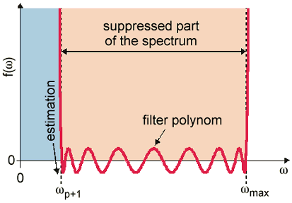
The highest frequency of the eigenmodes can
be estimated automatically if you do not already know the value of this
frequency. Therefore the eigenmode solver runs
a fast calculation with less points but more modes to get a proper estimation.
These fast calculations may be repeated iteratively in order to increase
the accuracy of the estimation. This iterative enhancement of the estimation
accuracy of the highest frequency of the eigenmodes may also be done if
you set the estimation for this frequency manually.
In most cases it is sufficient to use the automatically
estimated value to obtain a sufficient good accuracy for the calculated
modes. In some cases a better accuracy can also be achieved by increasing
the number of iterations up to 5.
Please note that the above mentioned statements
do not apply to the JDM eigenmode solver methods, which are parameter
free.
Solver logfile
After the solver has finished you can view the
logfile by clicking
Manage Results  Logfile Logfile  in the main menu. The logfile contains information
about solver settings, mesh summary, solver results and solver statistics.
Under solver results, all calculated modes are listed with their frequency
and the numerical accuracy following the definitions below. in the main menu. The logfile contains information
about solver settings, mesh summary, solver results and solver statistics.
Under solver results, all calculated modes are listed with their frequency
and the numerical accuracy following the definitions below.
Example:
--------------------------------------------------------------------------------------------
Mode Frequency
|
Accuracy
|
|(Ax-x)/x|
max(e)
div(e)
--------------------------------------------------------------------------------------------
1 8.02724981695
| 1.51e-013
8.05e-006 2.29e-015
2 10.1781072579
| 8.41e-015
4.94e-006 7.53e-017
3 10.3554337227
| 1.90e-014
5.92e-006 4.23e-016
4 12.5109337728
| 7.97e-015
3.82e-006 2.41e-016
5 14.7562186034
| 2.15e-011
2.33e-006 1.16e-012
--------------------------------------------------------------------------------------------
Definitions:
1. |(Ax-x)/x|: This expression stands for |(A*x
- lambda*x)|/|x| which is the relative error in the eigenvalue solution
A*x - lambda*x = 0. The norm used is the L2-norm.
2. max(e): The same definition as for 1., but
the norm used is the infinity norm.
3. div(e): This gives the remaining divergence
of the field by summing up all divergences at the mesh points in the calculation
domain.
Unphysical modes
Sometimes a few modes are looking really weird
and have a poor accuracy. These are unphysical modes which are basically
shifted static solutions including charges. They can easily be identified
by a huge divergence error (see solver logfile, div(e)). They do not affect
the accuracy of dynamic solutions, you can just ignore them.
See also
Solver
Overview, Eigenmode Solver
Settings, Eigenmode
Solver Parameters, Eigenmode
Solver Specials (AKS), Eigenmode
Solver Specials (JDM), Eigenmode
Solver Specials (Tetrahedral)


HFSS视频教程
ADS视频教程
CST视频教程
Ansoft Designer 中文教程
|
