|
|
|
| 首页 >> CST教程 >> CST2013在线帮助系统 |
Mesh Generation OverviewAfter you have set up your model geometrically and assigned the appropriate power sources and boundary conditions, your model has to be translated into a computer accessible format. As already mentioned above, the FI method, which is the foundation of CST STUDIO SUITE, is a volume discretization method. Your calculation domain has to be subdivided into small cells on which Maxwell’s Grid Equations must be solved. CST STUDIO SUITE can use the FI formulation on orthogonal Cartesian grids or on tetrahedral grids. The mesh influences the accuracy and speed of your simulation, so it is worth spending some time on understanding this process.ContentsAutomatic Mesh Generation with Expert System Recommended Initial Hexahedral Discretization Local Mesh Properties for Hexahedral Mesh Local Mesh Properties for Tetrahedral Mesh Meshing Thin Conductors using Tetrahedral Mesh Hexahedral Mesh GenerationIn general, there are three ways to define a hexahedral mesh: manually, automatically and adaptively. We will introduce their principles briefly before discussing details of the implementation in CST STUDIO SUITE.
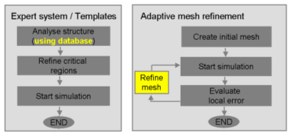
This following diagram shows the comparison of Expert System meshing based on project templates and adaptive mesh refinement. Mesh generation methods: Expert System based on project templates and Adaptive Mesh Refinement However, modifications to the structure force conventional mesh adaptation algorithms to start again from the beginning with each and every change of a parameter. Therefore the adaptive expert system hexahedral mesh refinement trains the expert system for a given structure. It can then maintain the mesh properties while the associated structure parts are slightly modified. You can increase your own expertise on mesh generation by analyzing the steps taken by the adaptive mesh refinement. You can use this knowledge to manually tune the mesh to increase the simulation speed for subsequent simulations. The strategies for mesh generation are quite different for high frequency problems as compared to low frequency applications. Automatic Mesh Generation with Expert SystemAfter this overview of meshing techniques, we go into the details of CST STUDIO SUITE’s hexahedral mesh generation for high frequency problems. The expert system uses lots of parameters controlling the mesh generation, having either local or global influence on the mesh. There are a few settings which you may frequently modify in order to obtain highly efficient meshes. Let's start with the most important global ones:
Please note: For low frequency applications the mesh will be automatically refined in substrates according to the corresponding material properties.
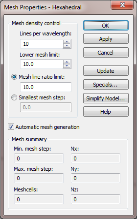
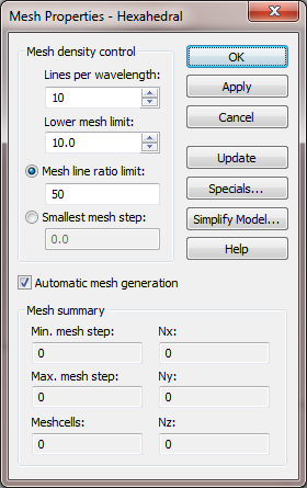
These parameters are also set by the Project Templates and the Adaptive Mesh Refinement. The first three settings can be changed in the Mesh Properties (Hexahedral) dialog:
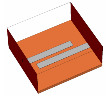
Please note: The Smallest mesh step determines the simulation speed! ExampleLet's start a new project, e.g. a simple coupled
microstrip line. The structure used for the following explanations is
shown in the picture below. To setup the project use File:
New and Recent
Now visualize the mesh by entering the Mesh View
(Home:
Mesh
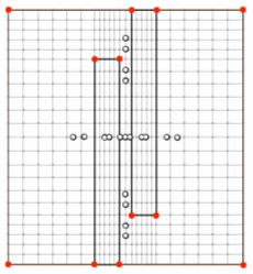
The picture above shows the grid being created using the default settings on the left side and using the Project Template’s settings on the right side. The red dots in the model are critical points (called fixpoints) at which the expert system finds it necessary to set mesh lines. They can be found on the bounding box, at the ends of straight lines, at circle centres and radii. In addition to these fixpoints, the yellow dots (white in the picture) show points where the automatic mesh generation improves the mesh density. Different settings of the global meshing parameters
explain the different grids seen above. For a closer look, open the Home:
Mesh
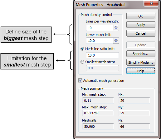
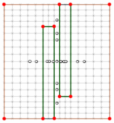
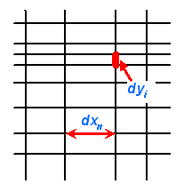
Lines per wavelengthThe Lines per wavelength parameter describes the spatial sampling rate of the field. A Lines per wavelength setting of 10 means that a plane wave propagating along one of the coordinate axes is sampled at least 10 times. The reduction of the wavelength when propagating through dielectric materials is taken into account here. Lower mesh limitThis setting allows you to define the maximum mesh step to be used for the mesh creation, regardless of the setting in Lines per wavelength. The maximum step width of the mesh is determined by dividing the smallest face diagonal of the bounding box of the calculation domain by this number. Mesh line ratio limit / smallest mesh stepThe Mesh line ratio limit parameter controls the ratio between the largest and the smallest mesh steps. Since the mesh lines are snapped to fixpoints, the smallest mesh step is usually determined by the structure’s details. If no lower limit is applied, this could result in very small mesh steps severely affecting the simulation performance (see section 4.2). Therefore, the Mesh line ratio limit parameter limits the creation of small mesh steps relative to the size of the largest mesh steps. In case of small details resulting in clustered fixpoints, mesh lines may not be placed at all fixpoints' positions. The following picture illustrates the meaning of the Mesh line ratio limit parameter: The smallest mesh step in this picture corresponds to dyi, whereas the largest mesh step is dxn. Therefore, the Mesh line ratio limit parameter needs to be chosen large enough to allow the mesh ratio to be at least dxn / dyi. Otherwise the two mesh lines at the ends of the mesh step dyi will merged together to a single line. It is obvious from the explanations above that the Mesh line ratio limit parameter has to be adjusted carefully. Too small settings of this parameter prevent the mesh from resolving small details. On the other hand, specifying very large values may result in very small mesh steps significantly affecting the performance of the simulation. As an alternative to the specification of the Mesh line ratio limit parameter, the size of the Smallest mesh step can also be specified directly as a global mesh setting. The mesh properties dialog box also shows some statistics about the total number of mesh cells, the smallest and the largest mesh step sizes and the number of mesh lines along each coordinate direction. Further settings of the expert system can be adjusted from within the Special Mesh Properties which can be displayed by clicking the Specials button in the mesh properties dialog box.
The General page contains an option Equilibrate mesh to reduce the local ratio between adjacent mesh steps resulting in much smoother density transitions. Furthermore, a special model for improved modelling of singularities at PEC or lossy metal edges can be controlled by the Use singularity model for pec and lossy metal edges button. Activating this feature significantly reduces the need for very fine meshes around such edges in order to achieve typically required accuracies. Due to the field singularities at PEC or lossy metal edges, the mesh usually needs to be refined around these edges. This is necessary even when the special singularity treatment is activated on the General page. The Refine at pec / lossy metal edges by factor option forces the expert system to automatically refine the mesh at critical edges by the given factor. The default setting is 2, but many of the Project Templates already increase this factor to 4 or more. The Consider pec / lossy metal edges along coordinate axes only switch determines whether the automatic refinement should be applied only to such edges. Since the refinement is also necessary along curved edges, this option should not normally be activated. Adaptive Mesh RefinementPerforming a single simulation does not provide any information about the accuracy of the solution. As mentioned in section 2.1, the FI method guarantees that the discretization error decreases with an increasing number of mesh cells. This property can be used to check the accuracy by refining the mesh, re-running the simulation and comparing the results. It is, however, important to find a good compromise between mesh density (affecting the simulation time) and accuracy.
The Project Templates try to adjust the global mesh settings to the particular kind of structure in order to obtain reasonable accuracy. The resulting mesh can then be used as an initial mesh for a subsequent mesh adaptation run. The following picture shows how the adaptive process is activated, e.g. for the transient solver by simply checking the Adaptive mesh refinement option:
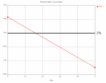
The Delta S quantity is defined as the maximum deviation of the S-parameters between two subsequent passes. This deviation is calculated by determining the actual distance between the corresponding curves in the complex plane rather than simply doing a frequency-by-frequency comparison. Small shifts in resonance frequencies therefore cause small differences only. Furthermore a weighting function is applied decreasing the contribution of errors at frequencies farther away from the center of the frequency band. The mesh adaptation stops once the S-parameters converge such that the Delta S value falls below a certain limit (2% by default). For the example consisting of two adjacent striplines, the mesh adaptation stops after 3 passes if the initial mesh were created using the Project Template. The mesh adaptation takes 6 passes using the default initial mesh.
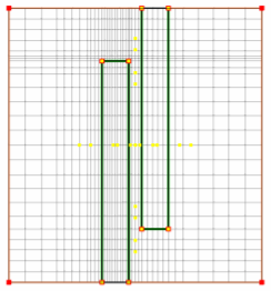
The mesh has been significantly refined along the PEC edges during the adaptive passes. In particular, additional mesh lines have been inserted between the conductors and at the edges of the stripline driven by the excitation:
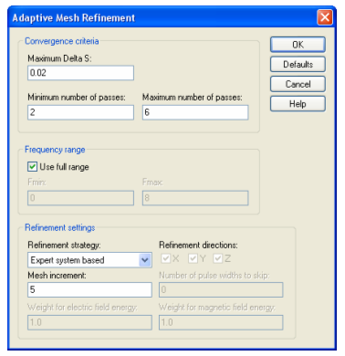
The adaptive meshing process can be controlled by setting its parameters in the Adaptive Mesh Refinement dialog box which you can open by clicking the Adaptive Properties button in the solver control dialog box.
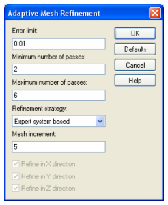
a) High frequency problem typeThe Maximum Delta S parameter determines the desired accuracy of the adaptive process. The adaptation will be terminated when the current Delta S value (see above) falls below this limit. You can also force the mesh adaptation to perform a Minimum number of passes by setting the corresponding value. Furthermore, the Maximum number of passes can be specified as a termination criterion. The mesh adaptation will stop once the specified maximum number of passes is reached regardless of the actual Delta S values. b) Low frequency problem typeThe Errorlimit parameter determines the desired accuracy of the adaptive process. The adaptation will terminate when the energy deviation between two consecutive passes falls below this limit. You can also force the mesh adaptation to perform a Minimum number of passes by setting the corresponding value. Furthermore, the Maximum number of passes can be specified as a termination criterion. The mesh adaptation will stop once the specified maximum number of passes is reached regardless of the actual energy deviation. Refinement strategyThe mesh adaptation process can be carried out by either an Energy based strategy or an Expert system based strategy. The Project Templates activate the Energy based method by default for planar structures.
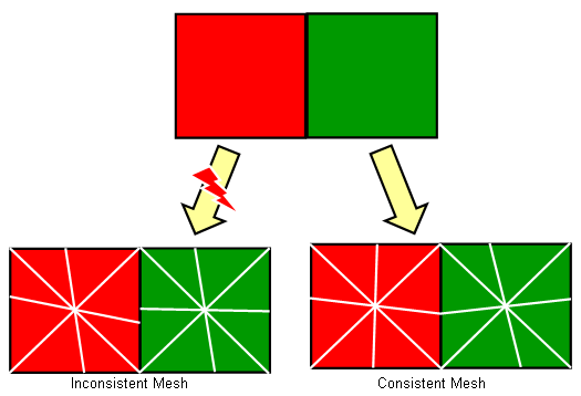
At the end of a successful expert system based mesh adaptation, CST STUDIO SUITE informs you that the expert system has been trained to yield accurate results for this structure. This means that it will not be necessary to start further adaptation runs with this structure since the quality of the mesh will be maintained even if you slightly change the geometry during parametric sweeps or automatic optimizations. Tetrahedral Mesh GenerationThe following section focuses on the principles of tetrahedral mesh generation. These general considerations apply to both high and low frequency problems. First, we explain the basic procedure of creating a tetrahedral mesh. Let us assume that a model consisting of several parts needs to be meshed. The solution methods require consistent meshes at the interfaces of different parts in order to set up the matrix equations correctly. The following picture shows two blocks touching each other at one of their faces. If the meshes were created independently for both blocks, the meshes might become inconsistent at the interfaces.
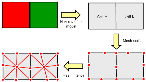
The typical solution to this problem is to create a ”non-manifold” simulation model first. This intermediate operation converts coincident faces from two solids to a single common double-sided face. Once this is done, the edges and faces of the model can be meshed in a first step. Based on this surface mesh, the volume mesh can then be created afterward. The non-manifold model guarantees that the surface meshes of neighboring solids are identical at their interfaces since they are built from the same surface mesh of the mutual double-sided face.
The following picture illustrates this procedure:
The tetrahedral mesh generation can be summarized as follows:
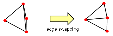
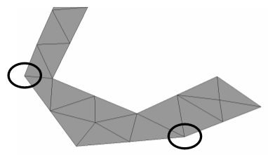
Once the initial volume mesh is created, its quality can be improved by mesh smoothing or mesh optimization. Mesh smoothing is an iterative scheme that moves the mesh nodes in order to improve the quality of the tetrahedrons. In contrast, mesh optimization is a technique that swaps edges and faces and reconnects them to form better quality tetrahedrons. The following picture shows a 2D example of how mesh optimization can improve mesh quality:
The tetrahedral mesh will be automatically created
whenever a solver is started requesting this type of mesh. However, in
order to visualize the mesh before running a simulation, you can enter
the mesh view at any time (Home:
Mesh Since the creation of the tetrahedral mesh is a
computational expensive task, the mesh is not automatically updated after
each change. You can force a mesh update by clicking the Update button
in the mesh properties dialog box or by choosing Mesh:
Mesh Control
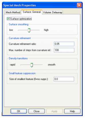
The global meshing parameters such as Steps per wavelength and Min. number of steps correspond to the Lines per wavelength and Min. number of lines settings for the hexahedral mesh generation. Refer to the corresponding sections above for details concerning the meaning of these settings. It is important to note that the high frequency tetrahedral mesh based solver uses a second order technique. Therefore, the default setting of 4 steps per wavelength corresponds to the 10 lines per wavelength default setting used for the hexahedral mesh creation. The tetrahedral mesh generation can be further controlled by parameters specified in the Specials dialog box. This dialog box contains three pages in order to influence surface mesh generation and volume mesh generation, respectively:
On the Surface mesh tab, the Surface optimization option and the Surface smoothing should normally be kept at their defaults. The Curvature refinement parameters control the quality of the approximation of curved faces by the surface mesh.
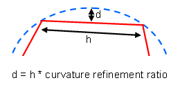
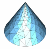
The Curvature refinement ratio specifies the ratio of the maximum deviation (d) of the surface mesh from the actual shape of the structure divided by the edge length (h) of the surface triangle (as shown in the picture above). Smaller values lead to better approximations of curved objects. Typical values are between 0.01 and 0.1. Due to mesh refinement based on the curvature of the object’s faces, the mesh becomes infinitely dense at a structure’s singularities such as the tip of a cone:
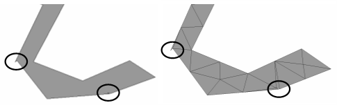
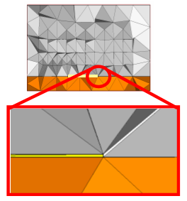
The Max. number of steps from curvature ref. parameter limits the amount of refinement due to the curvature of the model relative to the global mesh size specification. Large values allow a good approximation of high curvatures but will produce very fine meshes. Typical values for this setting are between 100 and 1000. Some imported models may contain small misalignments. The following picture shows such an example with a small gap and a small spike. Even if the tetrahedral mesh generation is able to properly mesh these types of geometry, this may nevertheless result in unnecessarily fine meshes:
Small structure details (”features”) can be suppressed by setting the Size of the smallest feature. If this value is set to zero, all details will be meshed. If a value greater than zero is specified, all features below this size will be suppressed as shown in the next picture:
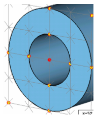
The Volume mesh tab contains parameters to control the volume mesh creation stage. The Volume optimization and Volume smoothing options should normally be kept activated. The Quality enhancement slider allows you to adjust how quickly the mesh changes between regions of different mesh densities. Smooth transitions result in good mesh quality but also increase the number of tetrahedrons in the mesh. The default setting is a good compromise for many cases and can usually be kept. Recommended Initial Hexahedral DiscretizationThe purpose of this section is to provide guidelines for the discretization of some typical types of structures using hexahedral meshes. We also recommend visiting a special training class on this topic. Please contact your support center for details. Coaxial StructuresThe following picture shows the coarsest recommended discretization for a coaxial structure as it may, for example, be used as initial mesh for adaptive mesh refinements:
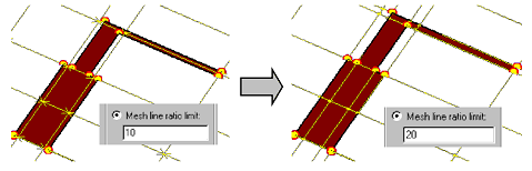
Make sure to adjust the Mesh line ratio limit parameter so that you have mesh lines at the center of the coaxial structures as well as at the inner and outer radii. Planar StructuresPlanar structures are usually quite sensitive in regard to meshing. We strongly recommend using the corresponding Project Template to adjust the meshing parameters to this type of structure. One of the most critical settings is the choice of the Mesh line ratio limit parameter. The expert system automatically identifies the small thickness of the conductors and avoids snapping the mesh lines to these tiny steps. Therefore, the Mesh line ratio limit can normally be chosen relatively large. However, sometimes planar structures have small distances between structure edges in the metallization planes. In such cases, it must be carefully decided whether to place mesh lines at these positions. Please note: The identification of conductor thickness as described above is only performed when the Merge fixpoints on thin PEC and lossy sheets setting is activated on the Fixpoints page of the Special Mesh Properties dialog box. This option is automatically set by the Project Templates for planar types of structures. The following picture shows a microstrip step (two microstrips with slightly different widths connected to each other):
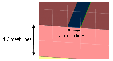
The picture on the left shows a mesh with a Mesh line ratio limit of 10. In this case, the mesh is not able to snap to the edges of both line segments, which results in poor discretization of the step. The picture on the right illustrates that the mesh lines can snap to the geometric details when the Mesh line ratio limit parameter is increased to 20 in this case. We strongly recommend that you inspect your mesh carefully and, in case of unwanted merging of mesh lines, increase the Mesh line ratio limit parameter accordingly. Furthermore, we recommend using at least 1-2 mesh lines across the width of the microstrip’s top conductor and 1-3 mesh lines along the height of the substrate.
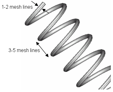
Helical StructuresThe following picture shows the recommended initial discretization for a helical structure:
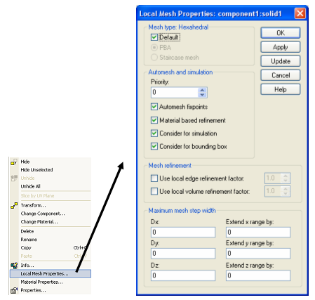
We recommend using at least 1-2 mesh lines across the diameter of the helix’s cross-section. Furthermore, 3-5 mesh lines should be used along the helix’s axis in between the turns. In cases where the diameter of the cross-section is very small, you should also consider modeling the helix as an infinitely thin PEC wire. Mesh TuningSo far we have discussed how to obtain simulation results and how to check their reliability with minimal effort spent on the meshing process. If you now feel confident with the global parameters and switches, let's go on to improve the mesh with respect to simulation time and memory requirements. Please note that there is an additional section on Transient Solver Performance Improvements . Local Mesh Properties for Hexahedral MeshUntil now we have discussed the approach to creating a mesh and studying the convergence by setting only a few parameters. CST STUDIO SUITE offers further useful ways of influencing the mesh, which can be used to save mesh points and thus decrease simulation time. After selecting one shape and pressing the right mouse button, you can open the Local Mesh Properties dialog box from the context menu:
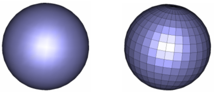
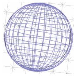
This dialog box contains a couple of shape specific settings which are discussed below. Automesh fixpointsIf the Automesh fixpoints option is switched off, CST STUDIO SUITE will not use any fixpoint of the particular shape. This option is sometimes useful when dealing with imported geometries. Let us now assume that you imported a sphere, but instead of an analytic description (left side), you got a faceted representation of it (right side):
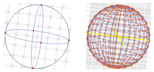
Although this is not a bad approximation of the sphere’s geometry, it is obviously not perfect. The CST STUDIO SUITE mesher always tries to model the shapes exactly as they have been defined. As a result, it will mesh this faceted approximation with fixpoints at the end of every straight line. And as you see below, instead of a very efficient grid representation (left), you end up with an unnecessarily large number of mesh points (right):
In case of a simple sphere, a reconstruction can be easily carried out, but in general you will need to keep your imported geometry as is. Switching off the Consider for automesh option will result in a representation as shown in the picture below:
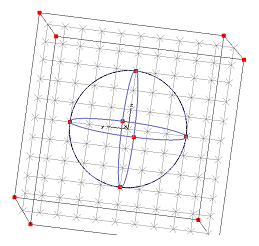
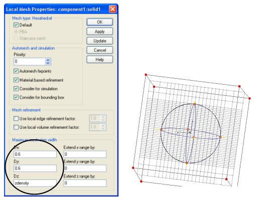
Now no fixpoints have been generated for the faceted sphere which leads to a more efficient mesh representation of the object. This option is also useful if your imported geometry is flawed because fixpoints are usually located at the most critical points of a geometric object. You should consider using this option if your structure contains an object that forces a lot of additional mesh lines but does not contribute much to the field solution to your problem. Maximum mesh step widthThis option allows you to locally increase the mesh density. This is important if you want to maintain a coarser grid in the peripheral regions but accurately sample the fields in the area of interest. For simplicity, let us again consider the sphere with its default mesh:
If we want to refine the mesh in the sphere’s volume, different values can be assigned to the three spatial directions in the Maximum mesh step width frame. You may also make use of parameters (e.g. zdensity = 0.3 here).
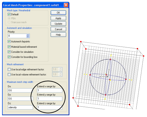
Especially in the case of PEC objects, the adjacent surrounding space is even more important than its interior. CST STUDIO SUITE offers the possibility to simply extend the volume within which the special settings will be applied:
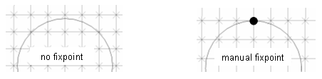
PriorityThe Priority setting determines a weight for the fixpoints of one geometrical object compared to another. If two fixpoints of different objects are so close together that the ratio limit does not allow the resolution of both of them, then a mesh line will be snapped to the point with the higher priority. Mesh typeThe type of structure representation can be individually determined for every object. The Default setting means that the global setting is taken, as chosen in the global Mesh properties, Specials dialog box (usually PBA(R)). For corrupted import data, where the healing algorithm failed, or for very large and complex CAD imports, switching to the standard staircase mesh might be helpful. Manually set fixpointsAs explained above, too many fixpoints can be avoided by switching off the Consider for automesh option. As a result, the fixpoints at the circumference of the imported sphere are also missing. It is, however, possible to manually set fixpoints at arbitrary locations. The pick operations which can be used for structure generation create fixpoints when applied in the Mesh view:
Manually defined fixpoints are marked by blue dots and have the highest priority in the mesh priority scheme. Local Mesh Properties for Tetrahedral MeshIn the same way as explained above for the hexahedral mesh generation, the tetrahedral mesh generation allows you to set local mesh parameters for individual shapes:
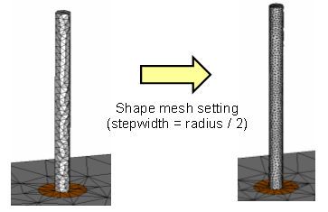
The mesh properties dialog box for a particular shape allows you to set a Max. stepwidth for the shapes volume, which then locally overrides the global setting. The tetrahedral mesh generation usually tries to generate tetrahedrons as equilateral as possible in order to obtain a high quality mesh. Therefore, the Max. stepwidth setting is a single value consistently applied to all directions. Now consider the following structure as an example:
The feeds are modelled by two cylinders with a relatively small radius. Using the default settings, the shape of the cylinders is not accurately represented by the tetrahedral mesh as shown in the following picture:
Specifying a maximum mesh step width for the two cylinders (e.g. half the radius) forces the mesher to sample the cylinders more accurately. As an alternative, the curvature refinement factor could be increased which would also yield a better resolution of the cylinders. The latter criterion, however, would be applied to all other shapes as well, which is not always the desired solution. Meshing Thin Conductors using Tetrahedral MeshMeshing thin conductors using a tetrahedral mesh can noticeably reduce the mesh quality. Note that due to the PBA(R) technique, this is not the case for hexahedral types of meshes. The following picture shows a cross-section of a mesh for a structure with a thin perfectly electrically conducting strip:
As can clearly be seen, the thin strip causes some of the tetrahedrons to become very flat, resulting in poor overall mesh quality. The latter will cause performance degradation since the convergence of the iterative equation system solvers strongly depends on the mesh quality. Furthermore, the convergence of the adaptive mesh refinement strategies is negatively affected by low quality meshes. As a rule, you should always consider whether the finite thickness of the conductors should be taken into account when using tetrahedral meshes. Whenever possible, you should model such conductors as infinitely thin which yields shorter simulation times. If you already have a model with finitely thick conductors, it may be easiest to use the Shape from picked faces operation which is explained in detail in the Planar Structure Tutorial. See alsoWhich Mesh to Use, Hexahedral Mesh, Tetrahedral Mesh, Surface Mesh, Mesh Problem Handling
HFSS视频教程 ADS视频教程 CST视频教程 Ansoft Designer 中文教程 |
|
Copyright © 2006 - 2013 微波EDA网, All Rights Reserved 业务联系:mweda@163.com |
|