|
|
|
| �� | |
| �� | |
| ��ҳ >> CST�̳� >> CST2013���߰���ϵͳ |
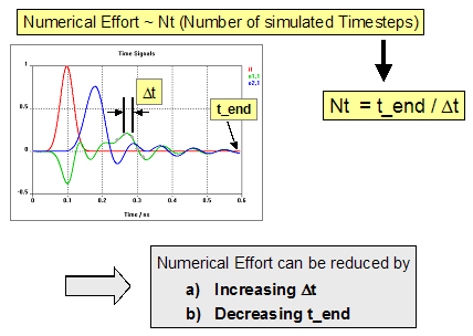
Time Domain Solver Performance ImprovementsThe transient solver uses an explicit time integration scheme, which implies that the solution is derived by simple matrix vector multiplications. This results in linear scaling of the numerical effort with the number of mesh points. Consequently the easiest way of reducing the simulation time is to use symmetry conditions, which reduce the number of mesh points by up to a factor of 8. However, there are some more possibilities to improve the solver performance, which will be discussed in the following sections.OverviewNumerical EffortTo better understand the following explanations, let's look at how the transient solver calculates S-parameters. The transient solver operates with time pulses, which can be easily transformed into the frequency domain via a Fast Fourier Transformation (FFT). The S-parameters can then be derived from the resulting frequency domain spectra:
For instance, a division of the reflected signal by the input signal in the frequency domain yields the reflection factor S11. Within just one simulation run in time domain, the full broadband information for the frequency band of interest can be extracted without the risk of missing any sharp resonance peaks. CST STUDIO SUITE automatically calculates the appropriate excitation time pulse from the frequency range setting. The default Gaussian-shaped pulse guarantees a nonzero spectrum in the frequency domain’s band of interest, which allows an accurate calculation of the S-parameters. Please
note: The number of frequency samples in Simulation:
Solver
Now take a closer look at the time pulses. The numerical effort and hence the total calculation time is determined by the total number of timesteps to be calculated. It can be reduced in two ways: a) Increasing the timestep width Dt or b) reducing the time t_end (see picture above). a) Increasing Dt
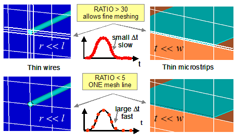
Because the time step �?span style="font-family: Symbol, serif; font-size: 10pt;">Dt is proportional to the smallest mesh step, it can be increased by avoiding unnecessarily small mesh steps. Here PBA allows the discretization of thin wires or thin microstrip lines without using a mesh step for the wire radius or the conductor thickness. As can be seen in the picture above, the Ratio limit setting controls the creation of small mesh steps. b) Decreasing t_end
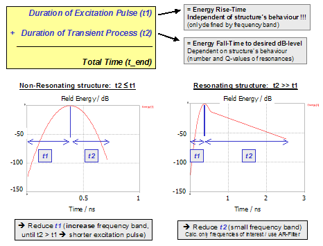
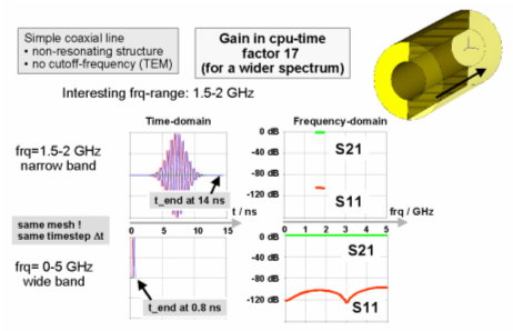
The total calculation time t_end is the sum of the duration of the excitation pulse t1 and the duration of the transient process t2. Depending on the structure’s behavior, it is useful to reduce either t1 or t2. Non Resonating StructuresFor non-resonating structures t_end can be shortened by reducing t1. This value is determined by the excitation pulse length and therefore directly influenced by the frequency range setting. The larger the bandwidth, the shorter the excitation time. In other words, for non-resonating structures you should always avoid very small frequency bands. This is demonstrated in the next picture for a coaxial line. By defining a wider frequency band, calculation time can be significantly reduced:
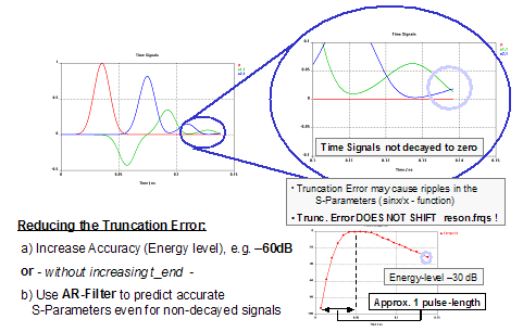
Please note that for models without a cut-off frequency (e.g. TEM and microstrip structures), DC should always be included in the frequency range since it shortens the excitation pulse by a factor of 2. For instance, the excitation time for a frequency range 0.01 ... 10 GHz is twice as long as for a range 0 ... 10 GHz. Regarding the choice of an appropriate upper frequency limit, two points have to be considered: you should avoid a) the excitation of resonances at higher frequencies and b) a large increase in the number of mesh points. However, if t_end is determined by the transit time of the signals, reducing t1 is not very efficient. That means that if the propagating pulse arrives at the output long after the excitation signal has vanished, the reduction of t1 will not influence the total time t_end significantly. Resonating StructuresFor resonating structures the reduction of t1 has no remarkable effect either since the total calculation time is dominated by the transient process t2. However, if you are just interested in the resonance frequency of a system, one possibility to reduce the calculation time t2 is to stop the simulation before the time signals have decayed to zero. This can be achieved by reducing the following: 1) the accuracy in the time domain solver control dialog box. (Default setting: -30 dB. In this case the solver stops when the remaining energy in the calculation domain decreases to -30 dB compared to the maximum energy.) 2) the maximum number
of pulses in the transient solver’s special settings (Simulation:
Solver If there is still a certain amount of energy left in the structure when stopping the solver, a ”truncation error” will appear. It causes ripples in the S-Parameter curves but does not shift the pole’s frequency.
In order to shorten the calculation time t2 for
resonant structures and avoid the truncation error, you can make use of
the Autoregressive Filter (Post Processing:
Signal Post Processing
General HintsSome other suggestions for increasing the simulation performance of the transient solver are the following:
See alsoAR-Filter Overview, Time Domain Solver Specials, Time Domain Solver Settings
HFSS��Ƶ�̳� ADS��Ƶ�̳� CST��Ƶ�̳� Ansoft Designer ���Ľ̳� |
�� |
|
Copyright © 2006 - 2013 ��EDA��, All Rights Reserved ҵ����ϵ��mweda@163.com |
|