• 首页
• HFSS教程
• ADS教程
• CST教程
• 射频工程师培训
• 微波仪器操作培训
• 天线设计培训
• 射频专业基础课

Ansoft Designer / Ansys Designer 在线帮助文档：

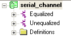
Nexxim Design Examples >
Nexxim SI Design Examples >
   Eye Analysis Example       

Eye Analysis Example

This example of a high-speed serial communications channel allows you to experiment with Nexxim Transient, QuickEye, and VerifEye analyses. This example focuses on modeling the effect of equalization on the performance of the channel.

The schematic for the channel with complete analysis and report setups is available in the Examples directory.

Open the High-Speed Channel Schematic project from its file in the Examples directory.

1. On the File menu, select Open Examples. The File Open window appears.

2. Open SI_Circuit, then select the file Serial_Channel.adsn. Click Open.

There are two circuits in the project:

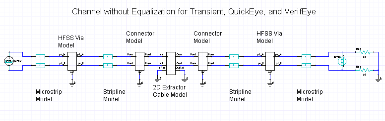
Click on Unequalized. The Schematic Editor displays the schematic:

This differential communication channel transmits first over surface-level traces, then through via connectors to buried traces, then through a cable connector to a cable, then back through cable connector, buried traces, via connectors, surface traces and termination on the receiver end.

The Eye Source at the transmitter end provides a controllable bit stream for both Transient and QuickEye analyses.

The left side of the circuit consists of the Eye Source, microstrip differential line pair, via connector, and stripline differential line pair.

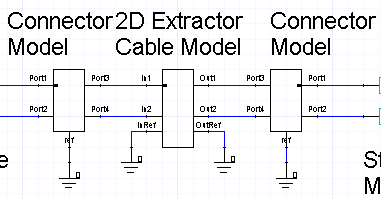
The center section of the circuit consists of the left cable connector, the cable modeled as a W-element, and the right cable connector.

The right side of the circuit consists of the stripline differential line pair, via connector, microstrip differential line pair, Eye Probe, and line termination.

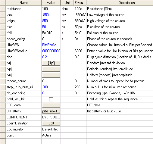
3. Select the Eye Source at the front end of the channel, and open the Properties window.

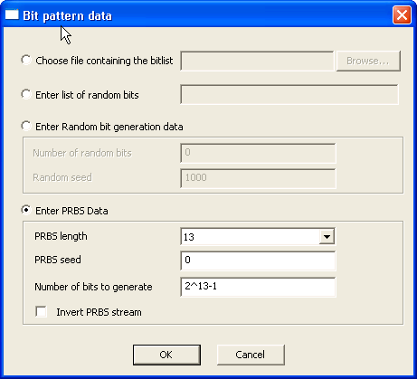
The source has a data rate of 6 GBits per second. Rise and fall times are 50 ps.

A 20% duty cycle distortion (DCD) will be applied to the transmitted signal.

4. Click on the Bit Pattern button to open the Bit Pattern Data dialog:

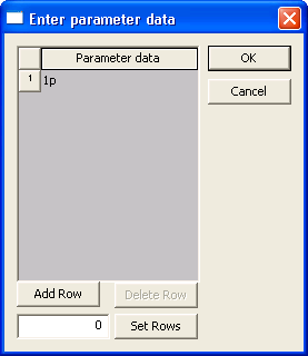
The pseudorandom bit source provides the bit stream for both transient and QuickEye analyses. Click OK to close the Bit Pattern Data dialog, and OK again to close the Properties window.

5. Click on the txrj button to open the Parameter Data dialog:

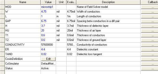
The source is set to transmit with a Gaussian jitter source using 1ps as the standard deviation. The jitter appears in all analyses.

6. Select the left Microstrip differential line pair and open its Properties window:

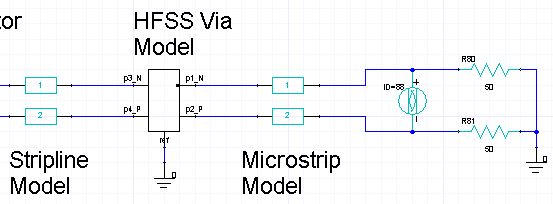
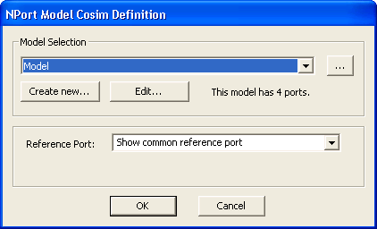
The two microstrip portions of the channel have the same parameters. The length of both segments is one inch.

7. The via connector is modeled with S-parameters. Click on the connector symbol and click Edit for the Cosim Definition.

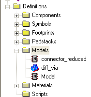
In the Project window, expand the Definitions folder and the Models folder:

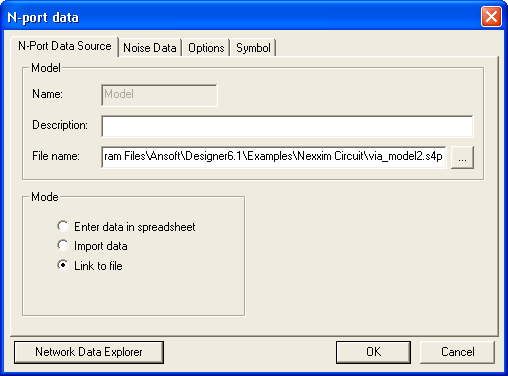
Click on the Model entry to open its N-port data dialog:

File via_model2.s4p contains the Touchstone data.

Both via connectors use this model.

8. Click on the left Stripline differential pair and open its Properties window:

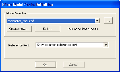
Both stripline segments use the same Parameter values. The length of both segments is five inches.

9. The cable connector is modeled with S-parameters. Click on the connector symbol and click Edit for the Cosim Definition.

The data is in the Models folder:

Click on the connector_reduced entry to open its N-port data dialog:

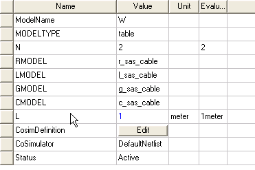
File connector_mode2.s4p contains the Touchstone data.

Both cable connectors use this model.

10. Select the Cable element and open its Properties window:

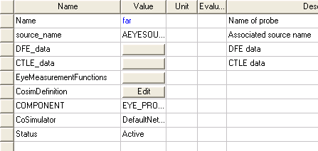
The cable is modeled with a W-element RLGC table model. The length is one meter.

The both ends of the channel uses the same elements.

11. Select the Eye Probe and open its Properties window:

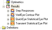
No receive equalization is set up in the probe. The next step is to simulate the circuit without equalization.

12. The project has setups for Transient, QuickEye, and VerifEye analyses. Right-click the Analysis icon in the Project tree and select Analyze. This starts all three analyses. It takes a few minutes for all analyses to complete.

13. Open the Reports icon. Four reports are set up.

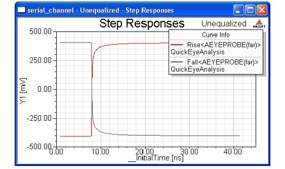
14. Double-click on the Step Responses report to open it:

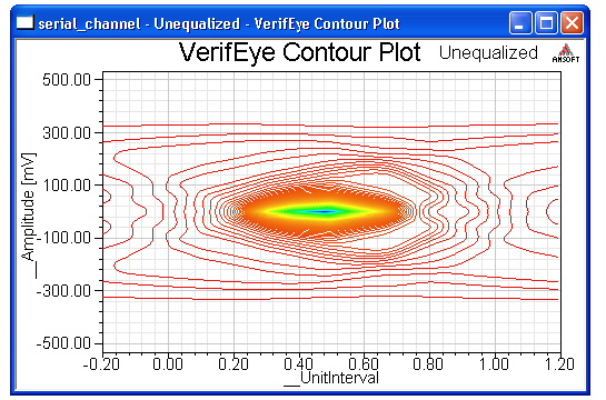
The step responses are symmetrical.

15. VerifEye calculates the channel response using a the channel parameters. Double-click on the VerifEye Contour Plot report:

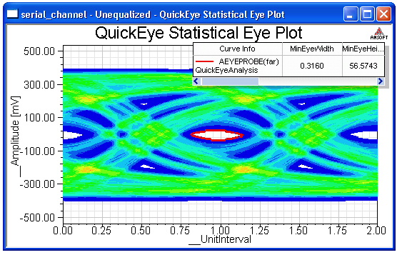
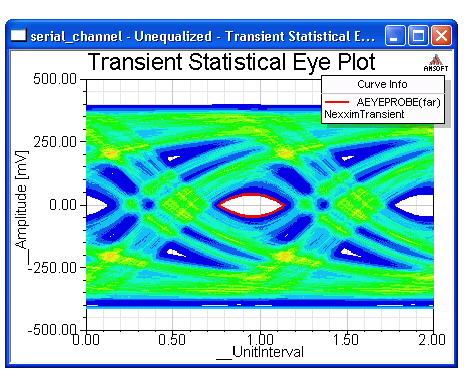
All the Unequalized plots show the negative effect of DCD and jitter on the eye opening.

16. QuickEye analysis convolves the impulse response of the channel with the bit pattern generated by the Eye source. Double-click on the QuickEye Statistical Eye Plot report:

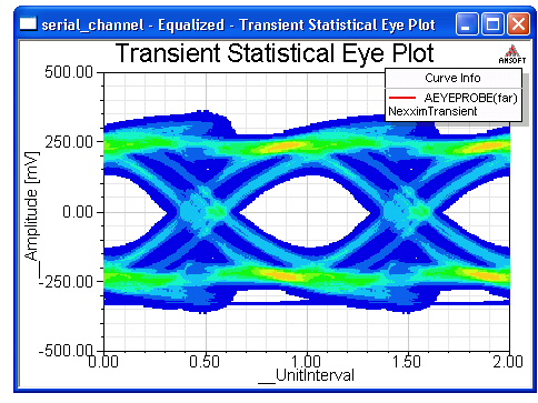
17. Double-click on the Transient Statistical Eye Plot report:.

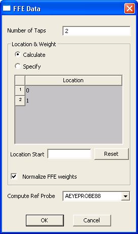
18. Now close the Unequalized schematic and reports, and open the Equalized schematic.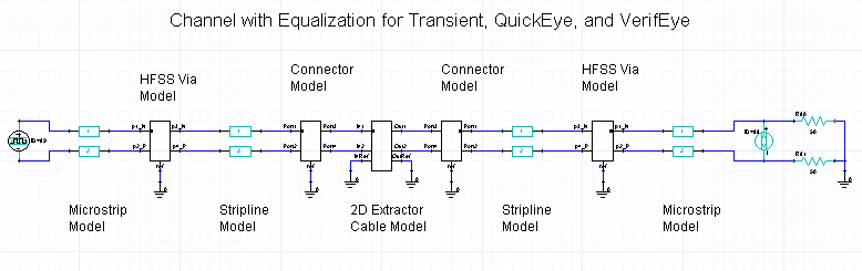

The circuit elements are the same, but the properties of the Eye Source and Eye Probe have been changed to add transmit and recieve equalization.

19. Select the Eye Source, open the Properties window, and click on the FFE_Data button to open the FFE Data dialog. Two taps of Feed-Forward Equalization are set up for the source:

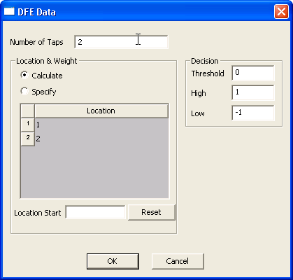
To disable Feed-Forward Equalization, set the number of taps to zero. To enable FFE, set the number of taps to an integer greater than 0.

20. Select the Eye Probe, open the Properties window, and click on the DFE_Data button to open the DFE Data dialog. Two taps of Decision-Feedback Equalization are set up for the probe:

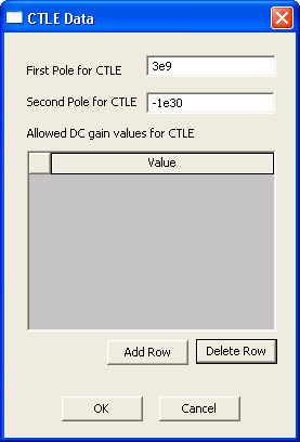
To disable Decision-Feedback Equalization, set the number of taps to zero. To enable DFE, set the number of taps to an integer greater than 0.

21. On the Eye Probe Properties window, click on the CTLE_Data button to open the CTLE Data dialog. Two pole frequencies for Continuous-Time Linear Equalization are set up for the source:

To disable Continuous-Time Linear Equalization, set the first pole frequency to zero. To enable FFE, set the first pole frequency to a suitably high value.

22. The Equalized circuit project has setups for Transient, QuickEye, and VerifEye analyses. Right-click the Analysis icon in the Project tree and select Analyze. This starts all three analyses. It takes a few minutes for all analyses to complete.

23. The same four reports are set up.

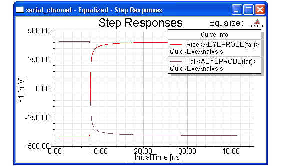
24. Double-click on the Step Responses report to open it:

The step responses are unchanged by the equalization.

25. Double-click on the VerifEye Contour Plot report. The effect of the equalization is apparent:

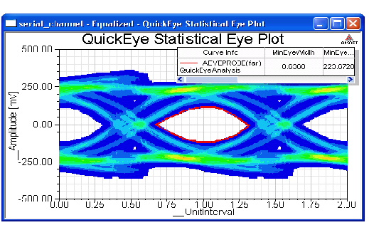
26. Double-click on the QuickEye Statistical Eye Plot report:

27. Double-click on the Transient Statistical Eye Plot report:.

Close the reports and the project when you have finished with them.

                HFSS视频教程                                      ADS视频教程                               CST视频教程                           Ansoft Designer 中文教程

      Copyright © 2006 - 2013   微波EDA网, All Rights Reserved    业务联系：mweda@163.com