|
|
|
| 首页 >> CST教程 >> CST2013在线帮助系统 |
Material Overview (HF)In CST MICROWAVE STUDIO, several different material properties are considered to allow realistic modeling of practical simulation problems. The two basic materials available are PEC (Perfect Electrically Conducting material) and Vacuum. Other more complex materials may be defined in the Material Parameters dialog. Each material is distinguished by its unique name and can be visualized in a selectable color and transparency.Considering linear behavior, in the frequency domain the dielectric and magnetic material parameters determine the ratio of the electric field and flux density and of the magnetic field and flux density, respectively:
In the following the description of the material is specified by its relative parameters with respect to the vacuum case. The vacuum permittivity and permeability are defined as
|
|
|
and |
|
. |
Consequently, the tangent delta value is given as the negative ratio between imaginary and real part of the complex permittivity or permeability, respectively:
|
|
and |
|
. |
|
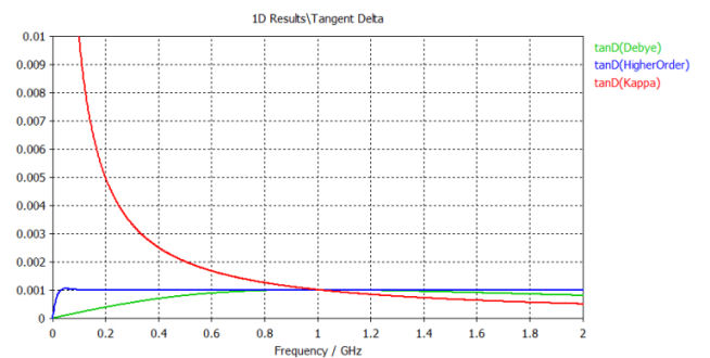
In general, every linear material behavior is described with help of the expressions above. Besides the special dispersive models explained later, different possibilities for loss definitions are available in CST MICROWAVE STUDIO. One definition is the following conductivity model:
where Accordingly to the general complex permittivity model
This model realizes a broadband constant conductivity, however, the corresponding tangent delta value is frequency dependent, as displayed in the right picture.
|
|
To realize an almost constant tangent value, or to set up a specific tangent delta curve, an internal dispersive first order Debye model (see below) will be fitted to the tangent delta input. The green curve on the right demonstrates the tangent delta dispersive behavior of such a model. Obviously, it is less frequency dependent than the conductivity model.
Higher order models for constant tangent value fitting are also available. They are specifically developed for low losses (low tangent delta value) and provide an almost constant broadband imaginary part. The model is described in term of a poles-zero representation such as that used for the General dispersion models (see below). The blue curve, corresponding to an order=7, demonstrates the high accuracy of this model.
Please note that no material exists in reality, providing a broadband perfectly-constant tangent delta value.
This
material type simulates the penetration of electromagnetic fields inside
a very good but not perfect electrically conductor by use of an internal
one-dimensional surface impedance model. This offers the possibility to
take the so-called skin effect into account without refining the mesh
for these materials. However, please keep in
mind that this model is physically reasonable only for a specific frequency
range, defined by the solid's dimension and its material properties: the
conductivity ![]() and the permeability
m
. As mentioned above, on one hand the material
has to represent a very good conductor, that means a material with a high
conductivity value or, in other words, a material with a high
tangent delta value:
and the permeability
m
. As mentioned above, on one hand the material
has to represent a very good conductor, that means a material with a high
conductivity value or, in other words, a material with a high
tangent delta value:
|
|
|
, |
|
. |
Obviously this defines an upper limit for valid frequencies, but on the other hand the frequency dependent skin depth of the fields

has to be smaller than the thickness d of the corresponding metal solid. This then defines a limit for the lowest applicable frequency:
![]()
using a weight factor of approximately 0.2.
Both constraints define together the valid frequency range for this material type, thus to take lower frequencies into account the material should be modeled applying a normal material type in connection with an electric conductivity. Consequently, for broadband simulations the frequency range should be split into two intervals.
Note that this kind of material type is also available as a boundary condition to suppress unwanted box resonances of the structure model.
To consider frequency-dependent material behavior in broadband simulations, a general representation consisting of superposition of first and second order model is available. Anyway the most common materials require up to second-order dispersion, as this model includes relaxation and resonance effects and is suitable as well for plasma or even for gyrotropic media. In each case the microscopic material behavior is represented by a macroscopic description of the permittivity or permeability in the frequency domain. Hereby the static parameter limit is indicated by the subscript 's' and correspondent to this the high frequency limit by infinity symbol.
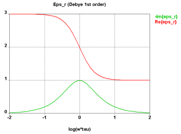
The relaxation process, also called first-order Debye model is characterized by the following formulation for the relative permittivity, containing the relaxation time t:
The second-order Debye model is a superposition of two different first-order models sharing the same high frequency limit.
The resonance behavior of a material is described by the Lorentz model, containing the resonance frequency w0 and the damping factor d:
![]()
|
|
|
|
Relaxation Process |
Resonance Process |
In the pictures above, the real and imaginary parts of the relative permittivity are shown. On the left a typical relaxation process is visualized by a Debye first-order dispersion model. The relaxation time determines the frequency range of significant changes. In contrast to this is a Lorentz resonance curve on the right, demonstrating the material resonance at the resonance frequency. Both models are also available for magnetic dispersions, i.e., for frequency dependent permeability.
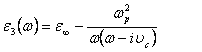
A special material behavior is described by the cold-plasma model, also known as the Drude dispersion model. This model describes the characteristics of media with two kinds of charge carriers. Furthermore, one kind (usually fixed ions in metal or slow ions in a plasma) is assumed to be stationary while the other kind (usually electrons) is allowed to move freely. Damping is obtained by elastic collisions of the moving particles with the stationary particles, described with help of the collision frequency nc. Considering the specific plasma frequency wp the correspondent relative permittivity is given as
It is also possible to model a dependency of the instantaneous plasma frequency wp from the local electric field. This dependency introduces some non linear effect to the material describing a non-uniform space dependent material. This non linear effect can further be described by a hysteresis loop effect (see the figure below).
The parameters to be specified are the specific plasma breakdown frequency wb, the electric breakdown field Eb and the plasma maintenance frequency wm.
From a very general physical model consideration it can be derived that the standard plasma frequency wp depends on the ion charge density N0 available in the plasma according to the formula
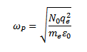
where qe is the electron charge, me the electron mass and e0 the vacuum dielectric constant.
According to this non linear model, the ion charge density depends on the local electric field. The complete hysteresis loop description follows.
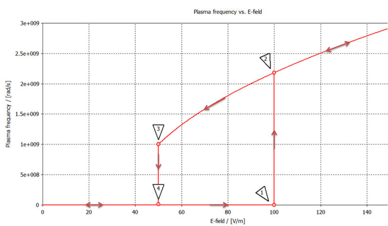
Starting from a zero field there is no ionization and plasma at all. When the field exceeds the so-called electric breakdown field Eb (see point 1 in the picture) an ionization effect ignites the plasma. The corresponding charge density results in the plasma frequency wb (point 2). As the electric field grows the ion charge density also grows linearly, such that the instantaneous plasma frequency exhibits a square root function.
Once the ionization has started, that is the electric breakdown has been overcome, the plasma ionization can be maintained for electric field down to an electric maintenance field Em which is generally assumed in the technical literature as half of the breakdown field Em=0.5 Eb. At the maintenance field Em the charge density results in the plasma frequency wm (point 3). If the electric field drops further below the Em value then the ionization cannot be maintained (point 4). The plasma condition does not hold any more resulting in a zero plasma frequency. In the picture below an example of the plasma frequency vs. the electric field is shown.
All dispersion models mentioned above can be described in form of a general polynomial formulation, modeled as a first or second order dispersion. This allows an efficient and accurate material description in its dominant physical behavior. Each first order model consists of just one real pole, a second order model includes a couple of complex conjugate poles and possibly one zero.
In case of a dielectric dispersion model of first or second order the corresponding expressions are given as
|
|
and |
|
, respectively. |
The same formulations hold also for magnetic material definitions. In both cases, the parameters of these general models can be directly defined in the Dispersive Material Parameters dialog or by applying an automatic fitting scheme to a list of material data values in the Dielectric/Magnetic Dispersion Fit dialog.
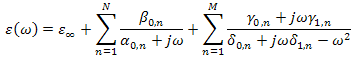
Furthermore, a superposition of the mentioned first or second order pole descriptions lead to a higher order material definition of the following general expression:
|
|
The parameters N and M represent the number of first and second order pole contributions and determine a material order of N+2*M. Such a material can either be defined by Visual Basic Language commands or again by applying a special automatic fitting scheme in the Dielectric/Magnetic Dispersion Fit dialog. Please note, that this dispersion definition is available to dielectric as well to magnetic materials.
|
The parameter for the first |
|
and for the second order model |
|
may be easily related to a physical interpretation, in term of poles and zeroes, resonance frequencies, quality factor and static (DC) gain (this quantity is also referred to as partial fraction gain)
In formulas, we may define:
first order model:
|
frequency of the pole |
|
|
static gain contribution |
|
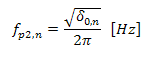
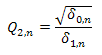
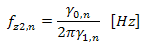
second order model (we are assuming a complex resonant model, otherwise the contribution may be further subdivided in two first order models):
|
resonance frequency |
|
|
quality factor |
|
|
frequency of the zero (if applicable) |
|
|
static gain contribution |
|
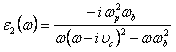
When a homogeneous magnetic biasing field is present in addition to the assumptions for the cold plasma, the effective material properties can be described by a gyrotropic permittivity tensor. If a z-directed biasing field is assumed, the correspondent permittivity tensor is given by
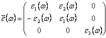
|
with the elements |
|
and |
|
|
|
and finally |
|
where |
|
. |
Here, the plasma frequency is again wp, and the cyclotron frequency wb arises from the circular trajectory of electrons with charge e and mass me in the constant biasing field B0. Damping is again due to the collision of the particles among each other, as described by the collision frequency nc.
Applying a static magnetic field to ferrite material causes a precession movement of the rotating electrons, which can be described by a frequency dependent and anisotropic permeability tensor. In fact, this material behaves strongly non-reciprocally and is significant for many microwave applications like circulators or one-way transmission devices. Such materials are called magnetic gyrotropic or simply gyromagnetic and are described by the following permeability tensor, assuming a magnetization above saturation in the z-direction:
|
with the elements |
|
and |
|
. |
Here, the Larmor frequency wl = G m0H0 (with H0 as the biasing static field) and the gyrotropic frequency wm = G MS are coupled to the magnetic flux density and saturation magnetization by use of the gyromagnetic ratio G = (g e) / (2 me). This factor is calculated from the Land茅 factor g in connection with the charge and mass value of an electron.
Furthermore the damping factor a, which was introduced by Landau and Lifschitz, describes the damping behavior of the precession movement. This factor can be determined from measurements of the resonance line width DH at a certain frequency w as
![]() .
.
Note that this material description is given in SI units. However, the ferrite parameters often appear in Gauss units referring to the input parameters Land茅 factor, saturation magnetization and resonance line width. Thus, for convenience, the Dispersive Material Parameters dialog offers both possibilities. In case you enter the material parameters in Gauss units, a reference frequency is needed to determine the damping factor a as described above.
For Time-Domain solver runs, a homogeneous biasing field can be assigned to each material.
For cases where the inhomogeneity of the biasing field needs to be considered, the Frequency Domain Solver with tetrahedral mesh features a convenient way to automatically calculate the magnetostatic field before the high frequency solver run. The solver then applies this biasing field to determine the ; varying material properties of the ferrites. Set up low and high frequency materials and sources in a single model, and then activate the Calculate static B-field for Ferrites option in the Special Frequency Domain Solver Parameters, and start the solver.
The material properties specified in the Dispersive Material Parameters dialog influence the initial mesh even if the magnetic field vector or the biasing direction and the Larmor frequency are overwritten with the corresponding values for the local magnetostatic field.
It is recommended to enter the material properties in the Gauss system, where the Land茅 factor can be specified directly. The C; frequency is proportional to the biasing field's magnitude, with the factor containing the Land茅 factor. The latter is then assumed to be equal to two if the material properties are given in the SI system (which approximately holds for many ferrites.)
In case of a nonlinear Material, the relationship
between the electric flux density ![]() and the electric field
and the electric field ![]() (similar representation holds for the magnetic flux density
(similar representation holds for the magnetic flux density ![]() and the magnetic field
and the magnetic field ![]() )
may be represented in a general form as
)
may be represented in a general form as
![]()
In this equation ![]() represents the linear contribution to the polarization whereas
represents the linear contribution to the polarization whereas ![]() and
and ![]() corresponds to the second order and third order
susceptibility.
corresponds to the second order and third order
susceptibility.
Finally with ![]() are labeled other sources of nonlinearity,
eventually of order higher than 3.
are labeled other sources of nonlinearity,
eventually of order higher than 3.
In general ![]() and
and ![]() are real second and third order tensors and therefore described
by 9 and 27 real values, so that a tensor product with the field is needed.
are real second and third order tensors and therefore described
by 9 and 27 real values, so that a tensor product with the field is needed.
This representation of the tensor may be simplified assuming an anisotropic but diagonal case, where only (the) 3 diagonal coefficients are needed. For an isotropic model a further simplification is possible, as only one real coefficient is required. Both simplified cases can be handled by CST MICROWAVE STUDIO.
In the following section we will concentrate only
on the isotropic case, so that ![]() and
and ![]() become real scalar values and the tensor product is easily performed
just computing the second and third power of the
become real scalar values and the tensor product is easily performed
just computing the second and third power of the ![]() field components.
field components.
In the anisotropic diagonal case the following considerations and notes holds for each of the three Cartesian field component, so that this case is also handled without further difficulties.
As a general important observation, please note that in case of nonlinear material no easy frequency representation is available for the field and fluxes. This is due to the nonlinearity which does not lead to an easy Fourier transform. All fields are therefore labeled as time dependent quantities and represented only in the time domain.
The transient solver of CST MICROWAVE STUDIO supports the following nonlinear material models (for further details see the Material Parameters - Dispersion page):
In the second and third order instantaneous nonlinear material model the electric flux is given by
|
|
and |
|
, respectively. |
where ![]() represents the linear contribution
to the polarization and
represents the linear contribution
to the polarization and ![]() and
and ![]() is the second or third order isotropic
susceptibility. The model is therefore completely specified by two real
values.
is the second or third order isotropic
susceptibility. The model is therefore completely specified by two real
values.
In this model the electric flux is given by
![]()
where ![]() represents the linear contribution
to the polarization,
represents the linear contribution
to the polarization, ![]() is the third order (infinity) isotropic
susceptibility and
is the third order (infinity) isotropic
susceptibility and ![]() a further nonlinear
polarization contribution.
a further nonlinear
polarization contribution.
This contribution arises when the medium changes its properties with the time showing a relaxation behavior, so that the effect of the finite response time of the material has also to be taken into account.
In particular for the Kerr effect the nonlinear polarization fulfills the following equations:
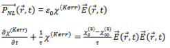
As seen from these equations the nonlinear polarization
follows a first order time differential equation - similar to a Debye
model - so that the Kerr effect is completely specified by the static
![]() and infinity
and infinity ![]() coefficient and the relaxation time
coefficient and the relaxation time ![]() .
.
Still the driving term to the differential equation
is ![]() . Therefore the nonlinear contribution belongs
to a third order nonlinearity.
. Therefore the nonlinear contribution belongs
to a third order nonlinearity.
In this model the electric flux is given by
![]()
where ![]() represents the linear contribution
to the polarization,
represents the linear contribution
to the polarization, ![]() is the third order (infinity) isotropic
susceptibility and
is the third order (infinity) isotropic
susceptibility and ![]() a further nonlinear polarization contribution.
a further nonlinear polarization contribution.
This contribution arises when the medium changes its properties with the time showing some resonance effects, so that the effect of the finite response time of the material has also to be taken into account.
In particular for the Raman effect the nonlinear polarization fulfills the following equation set:
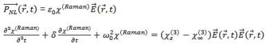
As seen from these equations the nonlinear polarization
follows a second order time differential equation - similar to a Lorentz
model - so that the Raman effect is completely specified by the static
![]() and infinity
and infinity ![]() coefficient
together with resonance frequency
coefficient
together with resonance frequency ![]() and the damping factor
and the damping factor ![]() .
Still the driving term to the differential equation is
.
Still the driving term to the differential equation is ![]() .
Therefore the nonlinear contribution belongs to a third order nonlinearity.
.
Therefore the nonlinear contribution belongs to a third order nonlinearity.
The non linear dependence of the field may be interpreted as a space-time variant material permittivity and permeability. In the general case we may write
![]()
where
![]()
From this equation it is clearly seen that the contribution of a second order nonlinearity
![]()
may produce both a positive and negative variation of the permittivity, depending on the field value, whereas the contribution of a third order nonlinearity
![]()
only produces a positive variation as it depends on the square of the field.
This has strong implication on the time step for a stable transient simulation. To see that remember that the Courant&endash;Friedrichs&endash;Lewy condition for the time step in one dimensional case reads
![]()
Therefore a negative value of ![]() (e.g.
in a second order nonlinearity) requires a reduction of the time step
simulation to enforce stability (see also Special
Solver Parameters &endash; General), whereas a positive one does not
restrict the stability margin.
(e.g.
in a second order nonlinearity) requires a reduction of the time step
simulation to enforce stability (see also Special
Solver Parameters &endash; General), whereas a positive one does not
restrict the stability margin.
Similar considerations may be applied to the Kerr and Raman case even if the analysis here is more complicated due to the governing differential equation.
In the transient solver (see Special Solver Parameters - Material) a monitor may be defined which stores the instantaneous equivalent eps and mue variation due to the nonlinearity. This provides a deep insight into the material properties and a great help for a fine tuning of the mesh and other simulation parameters such as the time step.
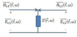
Surface impedances relate the tangential electric and magnetic fields on surfaces of bodies (solids or sheets) to which this material has been assigned. The effect of field inside bodies is described by equivalent currents on the surface of those bodies. Lossy metal, which is explained above, is an example for a surface impedance model.
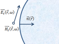
The exact relationship between electric and magnetic field at the surface impedance surface is governed by the formula
![]()
where (see the following picture)
![]() and
and ![]() are the tangential field components,
are the tangential field components, ![]() is the surface impedance value and
is the surface impedance value and ![]() is the inward pointing surface normal vector.
is the inward pointing surface normal vector.
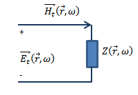
The surface impedance model leads therefore to the equivalent 1D transmission line model shown in the following picture, relating the electric and the magnetic field.
Corrugated wall surface impedance models are only available for the transient solver and the general purpose frequency domain solver with tetrahedral mesh. They are valid for electric field polarization that is perpendicular to the direction of the corrugation. The surface impedance is given by
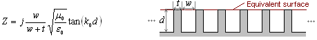
with the gap width w, the tooth width t (which should be less than one tenth of the gap width), and the corrugation depth d, which must be much larger than the corrugation width for the model to be valid. The number of corrugations per wavelength should be large, with ten per wavelength being the lower limit. There is a resonance in the effective material behavior when the corrugation depth is close to a quarter wavelength and its odd multiples, i.e.
The provided formula for the corrugated wall surface impedance is directly computed as it is by the frequency domain solvers. Anyway due to its high non-linear frequency dependence it is not straightforward applicable to the transient solver. To this purpose a specific fitting and representation of the impedance, based on a proprietary resonance expansion mode algorithm, will be automatically computed. The provided approximation leads to an accurate representation and results within the simulation frequency bandwidth.
Note: The validity of the corrugated wall surface impedance model for a given simulation cannot be checked by the solver. Therefore, it is mandatory to compare the results obtained with the equivalent material (i.e., the corrugated wall) to the full model at least once for a given problem type.
Ohmic sheet surface impedance models
are only available for the transient solver and the general purpose frequency
domain solver with tetrahedral mesh. Fields will not penetrate solid Ohmic
sheet bodies. Sheets, however, will have the same electric field on both
sides, that is they are considered as "transparent". The corresponding
1D transmission line model is the following, where the ohmic sheet value
![]() represents a "parallel shunt" element connecting the fields
at the two faces of the surface.
represents a "parallel shunt" element connecting the fields
at the two faces of the surface.
The following picture describes further the physical interpretation of the ohmic sheet material comparing it to a resistive brick. The geometrical dimensions for the brick and the sheet are specified by the length, l the height h and the width w.
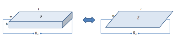
With this interpretation - and neglecting some high
frequency border effects - the seen resistance ![]() of the resistive brick (with conductivity
of the resistive brick (with conductivity
![]() ) is given by
) is given by
![]()
whereas the
same seen resistance in case of the ohmic sheet (with ohmic sheet value
![]() ) is
given by
) is
given by
![]()
|
The two models are therefore equivalent provided that |
|
This explains also why in the context of ohmic sheets the units is referred to as "Ohm per square", abbreviated "Ohm-sq", where the "per square" refers to a DC measurement with a voltage applied across a material sample.
The surface impedance is given by its resistance and reactance which are defined in correspondence of a reference frequency. The frequency domain solver computes a frequency independent model, i.e. resistance and reactance of the Ohmic sheet are assumed constant over the whole frequency range. This model is anyway somehow "non-physical" (see, for instance, to the so called Kramers&endash;Kronig relations) and cannot be directly simulated by the transient solver. Therefore the transient solver assumes a first order model for the frequency dependence of the complex impedance which exactly interpolates the user given resistance and reactance in correspondence of the reference frequency. The related formula (which is similar to that of the dispersive materials) is
|
where |
|
and |
|
are the complex impedances at zero and infinity frequency, respectively
|
and |
|
is the characteristic relaxation time.
Tabulated surface impedance models are only available for the transient solver and the general purpose frequency domain solver with tetrahedral mesh. The surface impedance is given in form of a table with its resistance and reactance tabulated versus frequency. Sheet bodies may be treated either as transparent or opaque. The former means that the electric field is the same on both sides of the sheet, while there is no direct coupling of the fields on front- and back-side of a sheet in the opaque case. The corresponding option is explained further in the Tabulated Surface Impedance dialog.
The frequency domain solver computes a linearly interpolated model across the given user points. It should be noted anyway that, depending on the user data, this model could correspond to a "non-physical" or "non-causal" behavior. For instance, possibly due to uncertainty or measurement errors, the so called Kramers&endash;Kronig relations could not be fulfilled. Therefore for the time domain simulation a rational fitting of the data will be performed, assuming a superposition of first or second order pole terms.
The internally fitted data are represented and stored in form of the impedance transfer function, using a higher (nth general) order material definition with the following general expression:
|
|
The parameters N and M represent the number of first and second order pole contributions and determine a material order of N+2*M.
|
The frequency dependent linear term |
|
corresponds physically to the contribution of an inductance. |
|
The parameter for the first |
|
and for the second order model |
|
may be easily related to a physical interpretation, in term of poles and zeroes, resonance frequencies, quality factor and static (DC) gain (this quantity is also referred to as partial fraction gain).
In formulas, we may define:
first order model:
|
frequency of the pole |
|
|
static gain contribution |
|
second order model (we are assuming a complex resonant model, otherwise the contribution may be further subdivided in two first order models):
|
resonance frequency |
|
|
quality factor |
|
|
frequency of the zero (if applicable) |
|
|
static gain contribution |
|
Perfect electric conductor (PEC), Ohmic Sheet and Lossy Metal material may be also specified as coated. This feature allows a compact representation of the material as a surface impedance without the need of meshing the coating itself. This would lead to fine details and much higher number degree of freedom and computational time / memory.
The layers attached to the original solid (PEC, Ohmic sheet or Lossy metal) describe the coating. Each layer should be of normal type, i.e. describing isotropic media material. Electric or magnetic dispersion is in any case allowed.
As a convention, the first defined layer is the nearest to the solid and the outer bound of the solid coincides with the outermost bound of the coating.
The coated material model works best for weakly curved structures (in terms of wavelength) and high frequencies. The coating material should have a rather high contrast to the surrounding material in terms of complex permittivity. So either the relative permittivity or the losses in the coating material should be large compared to the surrounding material.
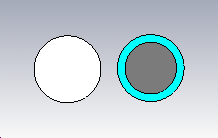
In the picture below two equivalent setups are shown. The left sphere is modeled by a single sphere and a coated material is applied. In the right setup a smaller metal sphere with a shell of coating material is used.
Please note that the outer bound of the solid coincides with the outermost bound of the coating, i.e. the radius of the coated sphere does not increase. In typical applications (for instance the RCS computation of an aircraft) and for electrically large simulations this is not an issue as the thickness of the coating is usually negligible compared to the size of the structure.
|
|
The frequency domain solver computes the material equivalent properties using standard impedance transformation formulas, starting from the basic solid type and adding successively the coating layers. It should be noted anyway that, depending on the user data, this model may lead to a "non-physical" or "non-causal" behavior. For instance, possibly due to uncertainty or measurement errors, the so called Kramers&endash;Kronig relations could not be fulfilled. Therefore for the time domain simulation a rational fitting of the surface impedance curve will be performed, following the same approach as for the tabulated Surface impedance model. The internally fitted data are represented and stored in form of the impedance transfer function using a higher (nth general) order material definition using a superposition of first or second order pole terms.
The transient time domain solver can handle materials with temperature dependent permittivity-, permeability- and conductivity-parameters of the normal and anisotropic material classes. A temperature dependent material definition consists of:
a reference to a previously defined temperature field import and
a table which defines a material parameter vs. temperature.
The transient time domain solver currently supports only temperature fields defined on a hexahedral mesh. If a temperature field produced by the tetrahedral based solver has been imported, an error message is displayed.
The temperature dependency curve can be defined in the Temperature Dependent Materials dialog, which is displayed by pressing the Properties... button. After definition the material table can be visualized as a 1D plot by selection in the navigation tree:
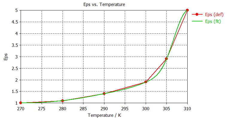
If possible a spline interpolation is computed with the given data, which will be visualized together with the user data. If the interpolated data is available the solver uses this curve for evaluation, otherwise the entered data is interpolated linear. After the transient solver has computed a material distribution, it is stored as a 3D result in the navigation tree.
Besides the mentioned electric and magnetic material properties also the density value of a can be defined. This is necessary to perform SAR calculation as a postprocessing step.
Modeller View, Material Parameters


HFSS视频教程 ADS视频教程 CST视频教程 Ansoft Designer 中文教程
|
Copyright © 2006 - 2013 微波EDA网, All Rights Reserved 业务联系:mweda@163.com |
|