|
|
|
| 首页 >> CST教程 >> CST2013在线帮助系统 |
Optimizer OverviewThe optimizer may be used to find optimal parameter settings for the modeled structure. Therefore, it is necessary to select the parameters that may be varied during the optimization process. The optimizer tries to minimize a function — the goal function. This function depends on the parameters selected for variation by the optimizer. Therefore, at least one goal must be defined that is evaluated while the optimizer is running. The goals for an optimization are always based on result templates. The optimizer tries to minimize the goals by varying the selected parameters.
Algorithm type There are four different types of local and three different types of global optimizers available. The local ones are the Trust Region Framework, the Nelder Mead Simplex, the Interpolated Quasi Newton, and the Classic Powell optimizer. The global ones are the CMA Evolutionary Strategy, a Genetic and a Particle Swarm optimization algorithm. By using a statistical model CMA Evolutionary Strategy improves it's performance without sacrificing it's global optimization approach. You may select the optimizer type from the Optimizer - Settings property page. More information about the optimization strategies can be found at the Optimizer - Interpolation of Primary Data page and on the Optimizer - Global Algorithm Settings page. Parameters The optimizer is a multidimensional optimizer. Thus, it is possible to simultaneously optimize several parameters. The parameters selected for optimization must be bounded by upper and lower limits. You may select the parameters for optimization from the Optimizer - Settings property page. If you select the Interpolated Quasi Newton optimizer, it is necessary to set the number of samples N per parameter. Thus, the parameter range defined by the upper and lower limits is divided into (N – 1) sections. Within each section the primary data is interpolated. Goals The optimizer needs at least one goal that is evaluated while the optimizer is running. The goal value is calculated for each parameter configuration the optimizer sets during the optimization process. The goal value effects the further parameter configurations of the optimization process. Goals can be defined from the Optimizer - Goals property page. Please note that if the sum or the maximum of all goal values evaluated while the optimizer is running is expected to be greater than zero. If it becomes less than or equal to zero, the optimizer finishes, assuming to have found the optimum. Information / Optimizer logfile While the optimizer is running,
information about the course of the parameter settings and the evaluated
goal values are displayed on the Optimizer
- Info property page. Additional information is summarized in
the optimizer logfile. You may display the contents of the optimizer logfile
after the optimizer has finished by clicking Simulation:
Solver In addition, the course of the parameter variation and the goal values may be plotted by selecting the respective entries in sub folders of 1D Results/Optimizer in the Navigation Tree. How to start the optimizer You can launch the optimizer
dialog box by choosing Simulation:
Solver Distributed computing It is possible to increase the performance of the optimizer by running the selected solver for different parameter configurations using several computers simultaneously. To enable this feature press the Acceleration... button on the lower edge of the dialog. For more information on distributed computing, see the distributed computing overview.
General information Optimization is a broad field. Almost any problem in science can be stated as an optimization problem and there are multiple use cases for using optimization inside the CST STUDIO SUITE. Unfortunately there is no optimization method which is best for all use cases and making the right choice depends on the particular problem. However the following guidelines should help to set up an optimization efficiently. Template Based Postprocessing: To allow virtually any result as target for an optimization the optimizer goal definitions always work on results created by the template based post processing. In addition to the generality of those results this has the advantage that all relevant results are stored for each evaluated parameter combination. After previously executed optimizations or parameter sweeps the results can be accessed by investigating the corresponding table results. Using sensitivity information: It is a well known fact that local optimization can be much faster if automatically calculated sensitivity information is exploited compared to approaches were this information is approximated by e.g. Finite Differences. From an optimization point of view it makes much sense to invest some time to model your system such that sensitivities are calculated directly by the numerical solver and can be exploited by the optimizer. To illustrate this a few definitions and results are shown from the waveguide junction that can also be found in the examples. For the described optimization the frequency domain solver with tetrahedal mesh was used. The goal of the optimization is to have small reflection at ports 1and small crosstalk to port 2. At the same time equal transmition to the ports 3 and 4 is desired. Those specifications can be defined in terms of four goal definitions referring to the corresponding result templates that load the amplitudes of the S-Parameters as can be seen in the pictures below.
Please not that the "move min" and "move max" operators were not used for the first two goal definitions because they do not feature the use of sensitivities. In order to use the automatically calculated sensitivity information the result templates corresponding to the goals have to be of the type "1D" directly loading S-, Y- or Z-Parameters.
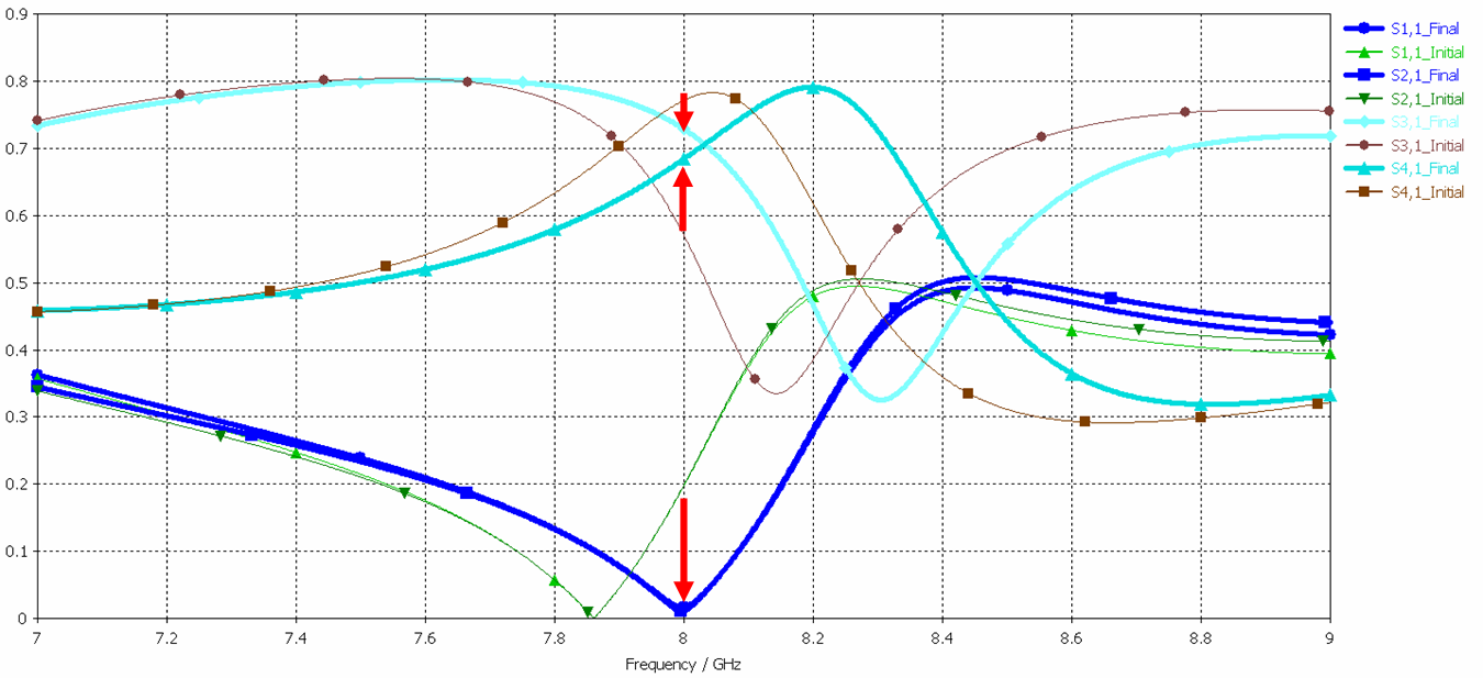
Five parameters were used for optimization: The height and radius of the disc and the gap were modeled with face constraints to produce sensitivities. The length and the width of the hole were modeled without sensitivities. To exploit the automatically calculated sensitivities the Trust Region Framework has to be used. By exploiting the sensitivities the optimizer was able to improve the S-Parameters as shown in the picture below by using 25 solver evaluations. The red arrows show the gained improvement. The final results with the solver option "calculate sensitivities" switched off looked almost identical but the algorithm had to use 68 solver runs to achieve this.
It's not possible to predict the acceleration that can be achieved using the sensitivity information but each parameter for which sensitivities are produced will yield a speed up of the optimization process. If the number of total optimization variables grows the achievable speed up will become even more significant. There is a message in the optimizer's info tab and logfile as well as the output window if sensitivities are exploited by the optimizer. The message will be printed after the optimizer's first successful solver evaluation.
See also Optimizer - Interpolation of Primary Data, Optimizer: Settings, Goals, Info, Optimizer - Global Algorithm Settings
HFSS视频教程 ADS视频教程 CST视频教程 Ansoft Designer 中文教程 |
|
Copyright © 2006 - 2013 微波EDA网, All Rights Reserved 业务联系:mweda@163.com |
|