The most common tasks performed in CST MICROSTRIPES are described here.
CST MICROSTRIPES is one of many products within CST STUDIO SUITE. First open the CST DESIGN ENVIRONMENT by double clicking on the icon on the Windows desktop, or by using the Start>Programs menu. Then in the Startup dialog that is displayed chose to open an existing project or create a new project. Select CST MICROSTRIPES for the new project if this is the product you want.
For all products in the CST STUDIO SUITE, the projects are stored in a CST file. When you open an existing CST file, the appropriate product from the SUITE will be launched.
The CST MICROSTRIPES window has three main areas. A Navigation tree, usually to the left, a display area where models and results are displayed, and a Message window to the bottom of the display. The user can control the position of the separate frames by dragging them to different position on the window. The views can be recovered, if deleted, by ticking them on the View menu.
Import a Project from CST MICROWAVE STUDIO
A CST MICROWAVE STUDIO project can be imported into CST MICROSTRIPES by pressing CTRL on the keyboard while clicking on the TLM solver icon.
Open a 2nd Project into CST DESIGN ENVIRONMENT
Multiple projects can be studied at the same time using CST DESIGN ENVIRONMENT. To open a 2nd or additional project, select File: New to create a new window to hold the additional project, then browse to the project you want. Selecting File: Open will by default load the project you want into the existing window.
Create a model for analysis
The steps that typically need to be done to create a model ready for analysis are:
• Set the frequency range and duration using the Model Parameters dialog.
• Define the geometry by importing an existing model or by using the Objects Toolbar, the Curves Toolbar and the Operations Toolbar.
• Assign material properties for the geometry with the Materials dialog.
• Review the Mesh Definition and Refine if necessary.
• Add any compact models to represent features such as Circuits and Wire Properties, Slots and Vents in an efficient way
• Choose the excitation type using the Ports or Excitations dialogs, or apply excitation directly on nodes in Circuits and Wire Properties
• Define the required Outputs
• Discretize the model and launch analysis. Some models will require postprocessing tool settings to be made.
Edit my geometry
The geometry of a model can be edited by double clicking directly on an object in the Build display if it is a simple construction. For more complicated shapes in the Navigation tree click on the Geometry view of a model to expand on the steps used to construct an entity. Then double click on any operation or primitive to edit it. Note that you will not be able to access the steps used to construct geometry if it was imported from another tool.
To perform operations on any object in the display, right click on that object (using Shift/Alt/Ctrl key will modify the right click behavior to select faces/edges or do a multiselect)
Two particularly useful features for constructing models are Variables which are defined at the top of the Geometry node in the Navigation tree, and Group for collecting entities together.
If you’ve hidden some objects from the view and want to get them all back, right click on the Geometry node in the Navigation tree and select to Show All.
If you have zoomed in too far, you can quickly reset the view by hitting the space bar.
Re-use one object in another model
Select File: Export to save the object as a sat file, then in another project use File: Import to load the sat file containing the object into that project.
Save my project with a new name
Select File: Saveas to create a copy of the project with a new name, and automatically load that project.
Analyse my model and view results
The results required for a model are defined using the output options of CST MICROSTRIPES and are listed in the Navigation tree after the model has been discretized.
To display the results, just double click on them in the Navigation tree. If you do not see any wanted results for a model in the Navigation tree, then outputs may not be defined for the model, or the model may not yet be discretized.
If a parameter sweep has been specified in the model definition, then the analysis will be queued for each variant of the model and launched sequentially. The list of models that still need to be analysed will be displayed at the bottom of the Navigation tree in the Job Queue.
The results for a model can be any or all of:
Time Domain
Frequency Domain
Space Domain
Transformed fields
Scatter Parameters
Shielded Cable
Time domain and frequency domain results are offered for output points, and voltage and current outputs on wires and circuits. These results are displayed in the graph plotter.
The space domain results are outputs defined over a region, such as electric field over the whole model at a specific frequency, or at an instance in time. The space domain results are displayed using the field plotter.
Transformed field results are obtained by transforming single frequency output generated within the mesh to the near field or far field. These include a near field cylindrical scan, near field cuts, far field radiation pattern, and far field cuts and conical cuts. The choice of which transformed fields are available for display depends on the appropriate analysis tool settings. For example, if the near field cuts are not requested in the tool settings for a project, they will not be displayed.
The scatter parameters can be obtained if the model contains ports.
The shielded cable solver is used to define the termination impedance for inner conductors of shielded cables.
Shielded cables are defined by attaching a cable material property to wires. The 3D Simulator will calculate the current on the ends of the inner conductors of all shielded cables, assuming the inner conductor terminations are matched. The Shielded Cable Solver can then take the model definition, and the time domain output from the 3D simulation, and calculate the current or voltage at the cable ends for different termination impedances.
By default the duration of the output of the Shielded Cable Solver is 10 times the duration of the 3D simulation. This is because using non matched termination causes the current on the inner wires to resonate and signals can take longer to decay.
Transients can be attached to models to excite a specific waveform, instead of using the default broadband excitation. These transients can be applied in the model itself, using Build, or they can be applied as post-processing options using the Tool Settings. If the transients are defined using the tool settings, then results with and without the effect of the transients will be available for the model.
To display the results for a particular result, just double click on the item in the Navigation tree. If the results have not yet been generated, or are out of date due to a model change or a change in the analysis tool settings, they will be automatically recalculated and displayed.
To launch all the analysis required to generate all the results for a project, right click and select Analyse All from Results in the Navigation tree.
Individual files generated during analysis can be viewed by selecting Edit: Options and ticking ’Show result files in Navigation Tree’.
![]() Change
Postprocessing Tool Settings
Change
Postprocessing Tool Settings
The tool settings are an important aspect of a project. They identify various input parameters required by the postprocessing tools. Each postprocessing tool has default settings, but the user should familiarise themselves with what these defaults are, and what other options are available.
The tool settings consists of a number of pages, one for each analysis tool that requires settings:
S-Matrix
Transients
Response Predictor
Fourier Transform
Near to Far Field
Shielded Cable Solver
If you make a change to a setting , then double click on the associated result to regenerate the results plot with the new setting applied.
View error messages and analysis output
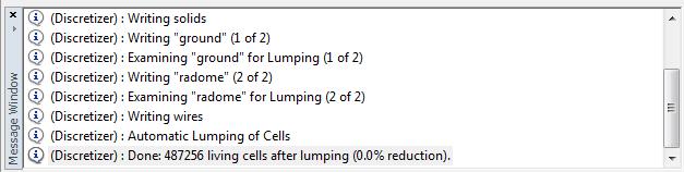
The Message Window is usually positioned at the bottom of CST MICROSTRIPES and is used to display errors, warnings and status messages generated by the analysis tools. This is where information will be reported about successful completion of a tool task, or why an analysis tool failed. It provides a log of the current modelling session.