PIC solver settings
Min. emitted current
If the minimum emitted current is enabled, emission occurs only if the absolute value of the emitted current is greater than the minimum. The minimum value means current per particle and not per source. Be always careful using this setting. Sometimes it is useful to activate this setting to avoid very small, negligible emitted currents and decrease computation time. The minimum current does not affect interface particles.
Note: Current per particle means the averaged current of one particle within the solver's time step. This current per particle is the quotient of macro charge and solver time step.
Min. emitted charge
If the minimum emitted macro charge is enabled, emission occurs only if the absolute value of the emitted macro charge is greater than the minimum. The minimum value means macro charge per particle and not per source. Be always careful using this setting. Sometimes it is useful to activate this setting to avoid very small, negligible emitted charges and decrease computation time. The minimum charge does not affect interface particles.
Neglect space charge effect
This setting will disable all space charge effects. In situations where relative small charges are tracked it is useful to switch off the current computation in order to speed up the simulation process (computing space charge currents is the most time consuming part of a PIC simulation).
In case this option is enabled, the PIC solver behaves like a transient tracking solver.
Sheet transparency
The sheet transparency is a filter for the particle's current, that means for the macro charge and macro mass. Thus the number of particle will not be reduced using the sheet transparency.
Percentage
Enter the sheet transparency for particles in percent. If the transparency equals 100%, no current is absorbed by the sheet. A transparency of 0% means that the complete current is absorbed be the sheet. If the sheet is not connected to the boundaries, it will get charged.
Import
Import an ASCII file to specify the cumulative distribution of the sheet transparency. This file has to consist of two columns, the first column is the energy in eV and the second column is the transparency. The transparency has to be monotonically increasing and between zero and one. (example)
Thermal coupling
Calculate power data
Calculate the time averaged collision power data and write it to a file. The data can be used to run a thermal solver calculation. Usually the calculated power is dependent on the solver run time or a user defined time interval.
Use solver simulation time
Check this box to use the complete simulation time for the computation of the average power data. To define a specific time interval for the power calculation deselect this check-box.
Start time
In case a user defined time span should be used to compute the power data, enter the start time here.
End time
In case a user defined time span should be used to compute the power data, enter the end time here.
Multipacting
Enable solver stop
If the multipacting detection is enabled and multipacting occurs, the PIC solver (and also the parameter sweep) will stop.
Intervals
Defines the number of intervals to be checked for exponential growth.
Interval width
Defines the interval width as time in units. The cutoff frequency of the low-pass filter is also defined by this value: Ω = 2 π / T
Exp. base
To detect multipacting the mean values (number of secondaries) of the intervals have to grow exponentially. The base of this exponential growth can be defined here.
Note
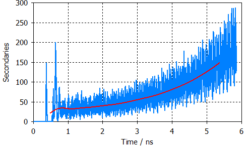
The multipacting detection is based on the increase of the secondary emitted particles. As this emission information is very noisy, it firstly has to be low-pass filtered. A typical filtered secondary emission curve could look like this:
|
|
|
Of course, the blue curve is the noisy secondary emission and the red curve the low pass filtered signal. For this example the interval width was set to 1 ns. |
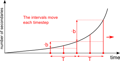
To get some information about the secondary emission, both signals shown above are available in the 1D result folder Solver Statistics [PIC]. The detection method checks the factor (slope) between the number of emitted secondaries at the interval boundaries and at the interval midpoints as shown in the picture below. Multipacting will occur if this factor is for all intervals greater than the user defined exponential factor and if the following necessary condition is fulfilled: Consider N as the number of source emission points. At least N secondary particles must be created at the midpoint in the right interval.
|
|
|
Visualization of the multipacting detection scheme. |
OK
Takes the current settings without closing the dialog box.
Cancel
Closes this dialog box without performing any further action.
Help
Shows this help text.
See also