Eigenmode Solver Overview

The eigenmode solver is used to calculate the frequencies and the corresponding electromagnetic field patterns (eigenmodes), where no excitation is applied. Loss free structures are supported (losses are available with the JDM method and hexahedral mesh, or by means of the perturbation method), without open boundaries.

The eigenmodes and their frequencies are the solutions of the eigenvalue equation

with the complex permittivity and reluctivity

$image\Eigenmode_Material.png$

respectively. The complex permittivity (reluctivity) is evaluated at a given material evaluation frequency. The complex angular frequency is related to the real angular frequency and the Q-factor by

$image\Eigenmode_ComplexOmega.png$ .

Which eigenmode solver method to use

The Eigenmode solver is available with hexahedral mesh and tetrahedral mesh.

With hexahedral mesh, two eigenmode solver methods are available and will be shortly described in the following: The Advanced Krylov Subspace method (AKS), and the Jacobi-Davidson method (JDM), which is capable to also solve lossy structures.

Normally, only a finite number of the lowest eigenmodes are needed. Therefore, the AKS solver uses a special filter polynomial to suppress the unwanted higher modes. The solver works in frequency domain using an iterative subspace method.

The AKS method depends on an estimation of the eigenvalue of the highest mode under consideration. This estimation is chosen automatically during an iterative estimation refinement process. If many of these passes are required, it might be advantageous to choose the JDM eigenmode solver, which is parameter free.

The solver time for the JDM eigenmode solver increases with the number of modes to calculate. Therefore, it is usually the method of choice if only a few modes are required. In many cases, the JDM solver is very robust, especially for multiple degenerated modes.

If the analyzed structure contains electrically or magnetically lossy materials which can be approximately described by a frequency independent complex permittivity or reluctivity, respectively, please choose the JDM solver, which automatically consider these materials. Consequently this method directly yields Q-factors for resonant structures, while Q-factors in loss free simulations are calculated by means of perturbation analysis as a post processing step (as done for the AKS solver or by choice for the JDM solver). In addition lumped L and C elements can be simulated with the JDM solver.

In case of tetrahedral mesh, one general purpose method is implemented and no choice of the method is to be made. A curved element order greater than One should be specified in the special tetrahedral mesh properties for a more accurate approximation of the geometry.

Areas of application

electromagnetic field distributions of modes at various frequencies
structure design by using the optimizer or the parameter sweep
external Q-factor calculation

How to start the solver

Before you start the solver you should make all necessary settings. See therefore the Eigenmode Solver Settings Overview. The eigenmode solver can be started from the Eigenmode Solver Parameters dialog box.

How the AKS estimation parameter influences accuracy

The most important parameter for a proper construction of the AKS filter polynomial is a good estimation of the highest eigenmode frequency to be calculated (see diagram).

$image\esolvov.gif$

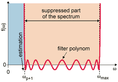
The highest frequency of the eigenmodes can be estimated automatically if you do not already know the value of this frequency. Therefore the eigenmode solver runs a fast calculation with less points but more modes to get a proper estimation. These fast calculations may be repeated iteratively in order to increase the accuracy of the estimation. This iterative enhancement of the estimation accuracy of the highest frequency of the eigenmodes may also be done if you set the estimation for this frequency manually.

In most cases it is sufficient to use the automatically estimated value to obtain a sufficient good accuracy for the calculated modes. In some cases a better accuracy can also be achieved by increasing the number of iterations up to 5.

Please note that the above mentioned statements do not apply to the JDM eigenmode solver methods, which are parameter free.

Solver logfile

After the solver has finished you can view the logfile by clicking Post Processing: Manage Results Logfile in the main menu. The logfile contains information about solver settings, mesh summary, solver results and solver statistics. Under solver results, all calculated modes are listed with their frequency and the numerical accuracy following the definitions below.

Example:

--------------------------------------------------------------------------------------------

Mode Frequency | Accuracy

| |(Ax-x)/x| max(e) div(e)

--------------------------------------------------------------------------------------------

1 8.02724981695 | 1.51e-013 8.05e-006 2.29e-015

2 10.1781072579 | 8.41e-015 4.94e-006 7.53e-017

3 10.3554337227 | 1.90e-014 5.92e-006 4.23e-016

4 12.5109337728 | 7.97e-015 3.82e-006 2.41e-016

5 14.7562186034 | 2.15e-011 2.33e-006 1.16e-012

--------------------------------------------------------------------------------------------

Definitions:

1. |(Ax-x)/x|: This expression stands for |(A*x - lambda*x)|/|x| which is the relative error in the eigenvalue solution A*x - lambda*x = 0. The norm used is the L2-norm.

2. max(e): The same definition as for 1., but the norm used is the infinity norm.

3. div(e): This gives the remaining divergence of the field by summing up all divergences at the mesh points in the calculation domain.

Unphysical modes

Sometimes a few modes are looking really weird and have a poor accuracy. These are unphysical modes which are basically shifted static solutions including charges. They can easily be identified by a huge divergence error (see solver logfile, div(e)). They do not affect the accuracy of dynamic solutions, you can just ignore them.