• 首页
• HFSS教程
• ADS教程
• CST教程
• 射频工程师培训
• 微波仪器操作培训
• 天线设计培训
• 射频专业基础课

Ansoft Designer / Ansys Designer 在线帮助文档：

System Simulator >
Frequency Domain Analyses >
   Single-Tone Frequency Domain Analysis >
       Sweep Domain Measurements           

Sweep Domain Measurements

Measurements available within the sweep domain include:

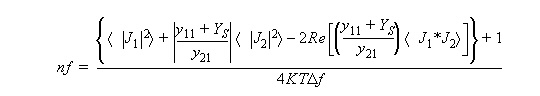
1. Port-to-port S, Y, Z, H, G and ABCD-parameters. For a system with N external ports, N×N Y (admittance)-parameters should be available. The S (scattering), Z (impedance), H (hybrid), G (inverse hybrid) and ABCD-parameters are simply obtained using matrix conversion techniques which convert the equivalent N × N system’s Y-parameters matrix Y_eq to the equivalent N × N matrix, assuming the default terminations of 50. The H, G, and ABCD parameters are calculated only for 2-port networks.

2. Port-to-port system’s noise figure (NF). NF is obtained by means of the system’s equivalent 2×2 Y matrix Y_eq and 2×2 noise correlation matrix J_eq, derived during the single-tone frequency domain analysis. This noise figure is given by:

where:

K = Boltzmann’s constant
T = Physical temperature in Kelvin
= Noise bandwidth (specified by the predefined Noise Bandwidth)
, where Z_s is always defaulted to 50

and all the Y and J parameters in the above expression are associated with the entries of the system’s equivalent 2×2 Y and noise correlation matrices Y_eq and J_eq.

Noise figure measurements may be obtained only for a system with two external ports, with one of the external ports being the input port. For a system with more than two external ports, all but two of the external ports must be terminated for noise figure measurements.

3. Signal to noise ratio SNR at the output port:

where:

N_i = KTf = -174dBm at 290Kelvin

S_i = Available input power

N_o = Available output noise power

S_o = Available output power

N_l = Noise power delivered to the load

S_l = Power delivered to the load

and nf is the expression for noise figure given previously.

Similar to the noise figure measurement, the signal to noise ratio may be obtained only for a system with two external ports with one of the external ports being the input port. For a system with more than two external ports, all but two of the external ports must be terminated for SNR measurements.

4. Noise power (NPWR) delivered to the load at the output port:

The noise power measurement may be obtained only for a two-port system with all other external ports terminated.

5. Port-to-Port Group Delay GD of the system is defined as:

where = The angle of S_ij(f) for the equivalent N-port system.

The above expression for group delay is approximated using finite difference. During single-tone frequency domain analysis, the system’s 2×2 equivalent Y-matrix Y_eq is obtained at the input carrier frequency f_c and the gain S₂₁(f_c) is extracted from this matrix by means of matrix conversion routines. Next, the frequency is slightly perturbed to
f = (1 + PERT)f_c and the system is reanalyzed to yield the perturbed gain
S₂₁(1 + PERT)f_c, then the above group delay expression is approximated by

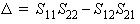
The group delay measurement may be obtained only for a two-port system with all other external ports terminated.

6. The stability factor K of a two-port system, which is obtained by means of the equivalent two-port S-parameters of the system

where

To obtain this measurement for a system with more than two external ports, all output ports except the desired output must be terminated.

7. The Output power (Pout) at all external output ports. For a system with M external output ports, the power delivered to the j^th load at the j^th external port is given by

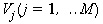
where the external port voltages are calculated as discussed below, and RL is the external port impedance.

8. The Output frequency (FO_j) at the j^th external output port. This output frequency is due only to the fundamental frequency of the input signal and does not include any harmonics generated within the system.

9. The voltage standing wave ratio VSWR_jj at the j^th external port. For a system with M external output ports:

10. The voltages at all external ports. For a system with N-external ports, these voltages may be obtained from solving the following set of linear equations:

where:

I_j = Current at j^th external port = equivalent input source current for j = 1and zero otherwise.

V_j = Voltage at j^th external port.

j = 1, 2, ... N

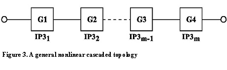
Y_eq = The N × N equivalent Y-parameters matrix of the system.

11. The third order output intercept power (OIP3). This measurement is applicable only to nonlinear cascaded systems (Figure 3).

For the general cascaded topology shown in Figure 3, the third order intercept output power is governed by the following equation:

where

G_i = The gain of the i^th element,

and

OIP3_j = if the j^th element is linear,

or

OIP3_j = value calculated from user- supplied nonlinear measurement data or user-supplied OIP3 parameter if j^th element is nonlinear

If the j^th nonlinear element is associated with a nonlinear measurement data (e.g., Pout vs. Pin) or sub-design, an attempt is made to extract the output power at the one-dB compression point (i.e. P1dB) from this data set, which is then used to calculate OIP3_j according to the formula discussed below. This calculated OIP3_j would override the user-supplied parameter OIP3 (if any).

12. The one-dB compression output power (P1dB): This measurement is applicable to nonlinear cascaded systems. P1dB is related to OIP3 through the following equations:

or

13. The saturated output power (Psat), applicable only to nonlinear cascaded systems, is calculated according to (refer to Figure 3 above):

where

G_i = The gain of the i^th element,

and

Psat_j = if the j^th element is linear,

or

Psat_j = value calculated from user- supplied nonlinear measurement data or user-supplied OIP3 parameter if j^th element is nonlinear.

If the j^th nonlinear element is associated with a nonlinear measurement data (e.g., Pout vs. Pin), an attempt is made first to extract the output power at the saturation point (i.e. the point where ). If this attempt fails, the above calculation will use the user-supplied Psat parameter for Psat_j (if any). Finally, if this parameter is not available, the Psat_j calculation will be derived from OIP3_j by one of the following formulas:

or

14. The dynamic range (DynRng) for cascaded nonlinear systems.

where OIP3 and N_o are the system’s 3^rd order intercept output power and output noise power, respectively.

15. Voltage Probes (VPs) and Power Probes (PPs) may also be placed anywhere inside the electrical system (prior to running the analysis). Each probe must be given a name by the user. Once the analysis is completed, these probes will be available in the Quantity field of the Traces dialog box. The voltage and power at the points where these probes are placed may be viewed for different swept values.

16. Return Loss (RTL_j) at the j^th external port. RTL_j = 1/|S_jj|

17. GFMN: Gain when the input impedance (Zopt) is used to achieve a minimum Noise Figure (FMIN). Available only in two port systems.

18. Real minimum Noise Figure power ratio (FMIN) is derived from fundamental noise quantities. Available only in two port systems.

19. Real equivalent noise temperature, . Available only in two port systems.

20. Real equivalent noise resistance ratio (RN) is derived from fundamental noise quantities. Available only in two port systems.

21. Real equivalent un-normalized noise resistance (RNU): . Available only in two port systems.

22. Complex optimum noise figure source admittance (Yopt) is derived from fundamental noise quantities. Available only in two port systems.

23. Complex optimum noise figure source impedance (Zopt), available only in two port systems.

24. Complex optimum noise figure reflection coefficient (GOPT), available only in two port systems.

                HFSS视频教程                                      ADS视频教程                               CST视频教程                           Ansoft Designer 中文教程

      Copyright © 2006 - 2013   微波EDA网, All Rights Reserved    业务联系：mweda@163.com