Modeling Nonlinearity using Polynomial Power Series — Ansoft Designer 7.0 在线帮助文档，Ansys Designer 教程

淘宝官方店推荐课程在线工具联系方式关于我们

	微波射频仿真设计 Ansoft Designer 中文培训教程 \| HFSS视频培训教程套装
	Agilent ADS 视频培训教程 \| CST微波工作室视频教程 \| AWR Microwave Office

Modeling Nonlinearity using Polynomial Power Series

It is always assumed that nonlinear measurements are obtained when the input and output ports of the nonlinear component are terminated in 50Ω. Nonlinear measurements of a two-port component typically include the AM-AM and AM-PM effects. This nonlinear relationship between S₂₁ and P₁ (the available input power) or, equivalently, between P_out and P₁ is represented by the following power series polynomials:

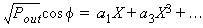
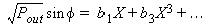
where

P₁ = the available input power from the source (with RS = 50Ω)

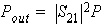= the output load power (assuming RL = 50Ω)

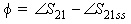
S₂₁_ss = the small signal gain.

The coefficients a₁, a₃, a₅,... and b₁, b₃, b₅,... are calculated using a least-squares curve fitting technique based on the user-supplied measurements P₁ - P_out data or P₁ - S-parameters data. For example, a set of coefficients can be obtained based on the following power amplifier P₁ - P_out measured data (in 50ohm terminations).

RTH_PA 2-port

POUT dBm

P1 dBm, FREQ = 900MHz

* P1	Pout	Phase (degrees)
5.00	25.68	88.75
7.00	27.67	88.75
9.00	29.66	88.75
11.00	31.64	88.75
13.00	33.61	88.75
15.00	35.56	88.75
17.00	37.48	88.76
19.00	39.35	88.76
21.00	41.16	88.76
23.00	42.86	88.75
25.00	44.38	88.71
27.00	45.65	88.66
29.00	46.53	88.76
31.00	47.17	91.85
33.00	47.50	97.08
35.00	47.66	102.81

Note

If the error obtained using the least squares curve fitting technique for the a and b coefficients exceeds 1e-5, an alternate approach based on cubic spline interpolation will be used to compute the output power level for a given input signal power

Note

If the input signal power to the nonlinear component exceeds the maximum supplied measured input power P1, the simulator will assume the last supplied output power entry in the measured data to be the saturation power.

Note

The above mentioned data is given at FREQ = 900MHz. Additional nonlinear measured data at other frequencies may be provided as well. The discrete time analysis is capable of locating the actual operating point using multi-dimensional data interpolation. For more information, please refer to the Nonlinear RF Component Models documentation.

If the user chooses to provide the nonlinear figures-of-merit (OIP3 or P1dB and Psat) instead of measurement data, the power series coefficients are approximated by

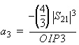
a_i = 0, i = 5,7, ...

b_i = 0, i = 1,3,5, ...

where:

S₂₁ is the linear small signal gain

OIP3 is the output power at the third order intercept point.

In this case, the simulations tend to be less accurate.


Copyright © 2006 - 2013 微波EDA网, All Rights Reserved 业务联系：mweda@163.com