|
微波射频仿真设计 |
|
|
微波射频仿真设计 |
|
| 首页 >> Ansoft Designer >> Ansoft Designer在线帮助文档 |
|
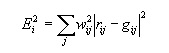
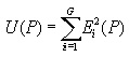
Optimetrics > Optimizers in the System SimulatorIn System analyses, you have the following choices of optimizer: Gradient, Random, MiniMax, and Levenberg-Marquardt. Gradient Search The Gradient search is based on a quasi-Newton algorithm which uses the exact gradient and an approximate inverse of the Hessian matrix of the Error Function to find a direction of improvement for each optimizable value. The search updates the approximate inverse of the Hessian using the Davison-Fletcher-Powell (DFP) formula or its complement. Appropriately combined with the gradient, this information is used to find a direction and an inexact line-search is conducted for each optimizable value. Successive iteration of this procedure, after each significant reduction of the Error Function value, continues the search for its minimum value. The first search direction is in the direction of the gradient vector. The term "line-search" means a search along a line in n-dimension space where n is the number of optimized values. Once a minimum is found in the first search direction, a second line-search in the same n-dimensional space is conducted. In the second and subsequent iterations, the direction of search depends upon the gradient vector, which is not the same as the overall gradient. The direction of the search is modified to accelerate convergence as a minimum is approached. When an Error Function minimum is suspected the search attempts to re-evaluate the direction based on the gradient alone, conducting a new line-search in attempt to find a path out of a potential local minimum. In practice the Gradient search is very efficient and when it is started from an initial point in the neighborhood of an Error Function minimum it finds the minimum very quickly. Even a slight gradient is sufficient to point the search in the correct direction. This strength is also the weakness of the method. The Gradient search is susceptible to local-minimum points. Once a local minimum region of the Error Function is arrived at, the Gradient search method may have difficulty in selecting optimizable values outside that minimum region. The number of iterations which are performed is specified before optimization begins. Each line search in n-dimensional space is referred to as an iteration. The number of iterations is actually the number of line searches. Each iteration may require several Error Function evaluations which in turn means that the circuit is re-simulated at all the optimization frequencies. The Error Function value decreases each iteration until, due to the circuit, optimizable values, goals or computation precision further reduction is not obtained and the optimization is terminated. In these cases further improvement may be achieved using a different search method. Optimization is always terminated if the value of the Error Function decreases to the termination limit which is 0.0 unless otherwise specified. The search is stopped as soon as the specified number of iterations for the optimization are completed. In this case additional iterations may be requested and a different search method may be used. Finally, the search may be aborted at any time using the appropriate abort function. Random Search The Random search arrives at new optimizable values following a Monte-Carlo approach. Starting from an initial set of optimizable values for which the Error Function value is known, a new set of values is obtained using a random-number generator within the applicable optimizable value ranges. The Error Function is re-evaluated and these optimizable values are retained if a decrease in its value is identified. The random-number generator may be randomized, to prevent any repetition, before the search begins. This is a trial and error process in which random search, eventually, finds an Error Function minimum that is near the global minimum of the Error Function. The Random search repeats this procedure for as many times as the number of iterations which are specified before the optimization is started. Each iteration may be successful in reducing the Error Function value. Unsuccessful iterations are not entirely wasted. Initially new optimizable values are drawn according to a uniform Gaussian distribution for each optimizable value. The optimized values are treated as independent Gaussian variables. After each iteration whether successful or not, the distribution is modified and becomes non-Gaussian. These modifications are made in order to skew the distribution towards lower Error function values and away from higher ones. The Random search tends to proceed in the direction of Error Function reduction but it is not restricted to such areas completely. More unsuccessful trials merely reduce the probability of selection of optimizable values in the respective regions. This feature improves the efficiency of the search without a risk of trapping the search in local minima. Each Random search iteration requires precisely one additional Error Function evaluation and is therefore less time consuming than an iteration of the Gradient search. However, some iterations may not be successful in reducing the Error Function value. These features allow the Random search to optimize the circuit even when it is started from an initial point which is far from an Error Function minimum or when its gradients are too small for the Gradient search. This search method is unlikely, however, to find the exact minimum point of the Error Function and may require many more circuit simulations than the Gradient search if the Error Function value surface is simple. Re-starting the search and randomizing the random-number generator may improve the search if many iterations are not successful. More iterations may be added after the search completes the number of requested iterations. Doing so allows the Random search to retain the accumulated modifications to the control Gaussian distributions mentioned above. The Error Function value decreases with each successful iteration until, due to the circuit, optimizable values, goals or computation precision, further reduction is not obtained. The Random search is prematurely terminated if the value of the Error Function decreases to the termination limit which is 0.0 unless otherwise specified. It may also be terminated if the search cannot find an improved solution using the weighted distribution built during the search process. Further improvement may be obtained by restarting the search, which will reset the distribution back to Gaussian. Finally, the search may be aborted at any time using the appropriate abort function. MiniMax Search The MiniMax method concentrates on the minimization of the largest weighted goal errors; minimizing the maximum contributions to the Error Function value. The MiniMax Error Function always represents only the worst case violation of the optimization goals, where the desired circuit response specifications are either most severely violated (in which case the Error Function value U > 0), or satisfied with the smallest margin (in which case the Error Function value U < 0). This Error Function may be defined in general as follows: U = MAXphrases {MAXgroups { MAXf {MAXgoals { wi*ei } } } } where U is the objective function to be minimized. ei is the discrete error function associated with a phrase at frequency f. wi is the weighting factor associated with ei. MAXgoals means the maximum value in the set over all goals of a phrase. MAXf means the maximum value in the set over all frequencies of a group. MAXgroups means the maximum value over all goal groups. MAXphrases means the maximum value over all optimization phrases. A MiniMax solution is one such that the goal specifications are met in an optimal, typically equal-ripple manner. The sophisticated MiniMax search method proceeds in two stages. In the first stage of the search, the MiniMax problem is solved using a linear programming technique and, in the second stage, the search employs a quasi-Newton algorithm which uses approximate second-order derivatives. A MiniMax iteration requires one evaluation of the objective function and its gradient, and therefore is less time consuming than an iteration of the gradient search. The objective function may occasionally be allowed to increase between iterations, but the final solution will have the smallest objective function value. Levenberg-Marquardt Search The Levenberg-Marquardt (L-M) minimization algorithm works on the least-squares error function:
where: P is a vector of N optimizable parameters G is the total number of specifications Ei(P) = wi [ ri (P) - gi ] is the weighted (wi) error between the computed response (ri) and assigned goal (gi) of the ith specification. For a single-valued goal, gi, and the LT or GT qualifier is used, it is assumed that Ei = 0 if the inequality is fulfilled. The same holds for two-valued goals when calculated response ri is within the range specified by the goal values.
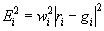
In the case of a complex goal, When circuit modeling goal is used then the error
where the summation is over all elements of S matrix. The L-M search makes use of two different strategies: the inverse Hessian method and the steepest descent method. The first one is similar to the method adopted in gradient search. It is commonly accepted as the superior strategy (in terms of speed and accuracy) if the current vector P is not far from a local minimum. The steepest descent method is more robust and it can make progress even far from minimum but at a cost of slow convergence. The L-M algorithm dynamically switches between the two strategies during the iterative search for minimum. The Hessian matrix, which is used in Newton phase of the L-M search, is not successively built up as in the gradient search. It takes advantage of the least-squares form of the error function U(P) and is estimated as H(P) = 2 JT(P) J(P) , where the Jacobian matrix of error vector E is defined as Jik (P) = d Ei (P) / d Pk , i = 1, … , G, k = 1, …, N and JT means J transposed. Such an approximation of H is always singular if the total number of specifications is less than the number of optimizable variables, G < N . Thus, for the original L-M algorithm the necessary restriction implies G > N. Implemented in the code is the modified L-M search that may overcome this limitation by a procedure called passivation. In this procedure, the N - G optimizable parameters are effectively eliminated by zeroing N - G smallest gradient components and corresponding elements in H matrix. A new selection of passivated variables is determined at each iteration of the L-M search. However, the passivation procedure consumes extra time and therefore it is not recommended to select L-M optimization method when G < N. On the contrary, if G > N, then the L-M search is very often better choice than the gradient search. Note: The error function used in L-M search differs from that used in gradient search and therefore their values (even if evaluated at the same P) may be different. At each step of the L-M search the error function and the Jacobian matrix J are calculated. From J, the corresponding gradient vector and Hessian matrix may be determined. Once they are updated, the Levenberg-Marquardt parameter and the search direction are calculated. The value of the parameter controls a smooth transition between the Newton and the steepest descent strategy. Having them both updated, the L-M algorithm finds a better minimum along the search line. After checking the conditions for termination, a new vector of optimizable variables P is calculated and the whole process repeats. Every iteration of the L-M algorithm requires a few error function evaluations. The L-M search stops when the local minimum is found, or when a number of performed iterations exceeds the predefined limit, or when the next guessed vector P lies outside the search region. As in the gradient search, once the L-M algorithm finds a local minimum it is trapped there and cannot perform further searches.
HFSS视频教程 ADS视频教程 CST视频教程 Ansoft Designer 中文教程 |
|
Copyright © 2006 - 2013 微波EDA网, All Rights Reserved 业务联系:mweda@163.com |
|
 .
.