|
微波射频仿真设计 |
|
|
微波射频仿真设计 |
|
| 首页 >> Ansoft Designer >> Ansoft Designer在线帮助文档 |
|
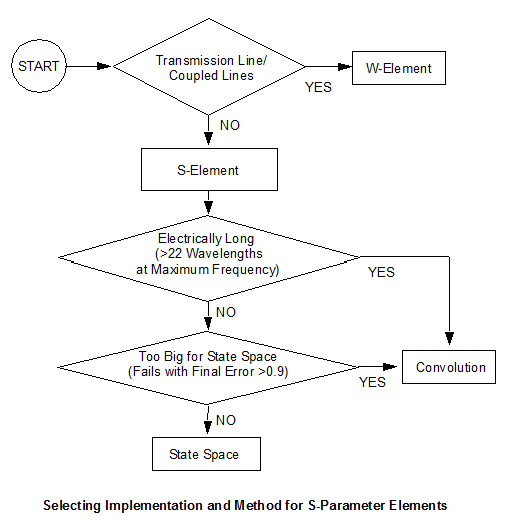
Nexxim Simulator > Troubleshooting S-Parameter IssuesThis topic shows how to select the correct S-parameter representation for your design and suggests ways to employ selected S-element options to minimize errors. Selecting the Correct Element and MethodThe flow chart below outlines the process of selecting the correct implementation for an element defined by S-parameters. The two main choices are between the S-element and the W-element, and then, for the S-element, between the default state-space representation and the convolution method.
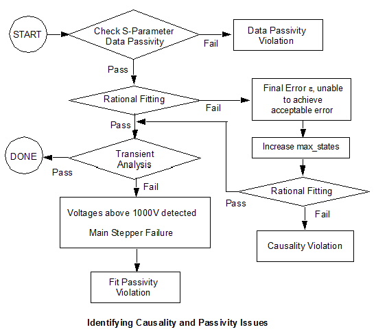
Selecting W-Element or S-ElementThe first decision is whether to use a W-Element or an S-Element. W-Element modeling exhibits fewer stability issues than S-element modeling. • When the S-parameter component to be simulated is a transmission line or a set of coupled lines, use a W-Element that points to an S-model. The S-parameter data must be well de-embedded. The S-model computes the unit RLGC or TABLE model for the W-element from the S-parameters. See Transmission Lines for details on the W-Element. • When the element has many ports, has a short electrical length, or is not a transmission line despite a long electrical length, use an S-Element to model the component in Nexxim. For processing S-elements, Nexxim uses one of two methods—state space or convolution. Selecting State Space or Convolution MethodNexxim must convert the frequency-dependent scattering parameters in the data to a numerical model that is suitable for simulation. The default representation, a state-space model calculated by rational fitting methods, is the best method for most applications. The alternative convolution method calculates the impulse response for the element and convolves the impulse response with the data during transient simulation. Convolution should be selected when: • The circuit is electrically long (greater than 22 wavelengths at the maximum frequency). • The circuit is too big for the state space representation. State space fitting fails with a message such as "Final Error e, unable to achieve acceptable error." The final error e, will be larger than 0.9 (e can exceed 1.0 in rare cases, but can never exceed 2.0). Refer to Convolution Method for details on setting the convolution options. See the S-Parameter Technical Notes for more on the State Space representation. Troubleshooting State Space IssuesState space models can exhibit passivity violations and causality violations. These stability issues may be present in the original S-parameter data or introduced by the numerical fitting methods. The S-Parameter Technical Notes provide much more detail on causality and passivity. The diagram below illustrates the process for diagnosing these two sources of error.
Identifying Passivity ProblemsPassivity violations can be detected in the original S-parameter data and rejected if they are serious. Mild passivity errors in the data may persist in the state space realization, and more serious passivity errors may be introduced by the fitting algorithms. State space passivity violations may result in errors during Transient analysis such as exponential growth of the voltages at the ports of the S-parameter block or time steps below minimum. Identifying Causality ProblemsCausality violations can lead to errors during the calculation of the rational fit to the S-parameter data. The final error (e in the diagram) indicates the magnitude of the fitting error. To verify that the problem is due to causality issues, increase s_element.max_states from 128 to 200 or 300 and retry. Increasing the maximum number of states per entry in the state space formulation works best when the S-parameter data are for a linear network rather than for a transmission line. The next sections give some suggestions for dealing with passivity and causality issues. Troubleshooting Passivity IssuesPassivity issues may be resolved by improving the initial rational fit or by applying a passivity enforcement algorithm to the state space matrices after the initial fitting. Improving the Rational FitImproving the rational fitting approximation can minimize passivity issues in some cases. • Set the s_element.column_fit option from default 1 to 0 or 2. 0=Fit each entry separately, then combine them at the end. 1=Fit one column at a time. 2=Do the entire matrix at once, using symmetry if present. Column_fit =1 and 2 work best for systems with many ports but with a short electrical length, like a chip package. • Increase the s_element.rational_fitting_iteration_limit option from default 2 to a higher number, 10 or 20. Increasing the maximum number of iterations improves the fit at the cost of simulation time. • Decrease the option s_element.reltol from default 1e-2 to 1e-3. Tightening the tolerance used for state space fitting may help with passivity problems, but could result in overfitting with non-causal data. Enforcing PassivityPassivity enforcement postprocesses the state-space matrices, making sure that the fitted S-parameters are passive. By default, no passivity enforcement is enabled. Three methods of passivity enforcement are available in Nexxim: an iterated fitting method, a convex programming method, and a perturbation method. All three methods add time to the simulation, but produce results that are accurate with respect to the original data. See the S-Parameter Technical Notes for details on these methods. • For most passivity problems, set s_element.enforce_passivity=7 to invoke the Iterated Fitting of Passivity Violations (IFPV) method. IFPV is the fastest of the three methods. • If the system has no more than ten ports (inputs and outputs combined), set s_element.enforce_passivity=1. Enforce_passivity=1 uses a convex programming method to enforce the passivity of the state-space mode. Enforce_passivity=1 automatically sets mor=1, since the passivity enforcement algorithm runs more quickly after model-order reduction. • If the system has more than ten ports (inputs and outputs combined), set s_element.enforce_passivity=6. With this setting, Nexxim uses a perturbation method for enforcing the passivity of the state-space matrices. Other Useful State-Space OptionsHere are some other S-element options that may be useful in dealing with state-space issues. Error ToleranceBy default, the error tolerance for S-parameter elements is based on the absolute difference between each entry of the fit and the corresponding entry of the S-parameter data. This scheme may not work well for some cases with very small off-diagonal S-parameter entries. • The option s_element.by_entry=1 sets Nexxim to treat the error tolerance as relative to the size of S-parameter matrix entry. Model-Order Reduction OptionBy default, the order of the state-space model is the order as calculated from the data. Reduction converts the state-space fit to a smaller one than the default, while maintaining the original accuracy. Reduction makes the transient simulation run more quickly, but at an up-front cost, so it works best when running a long simulation (one where the ratio of TSTOP to TSTEP is particularly large). • Set s_element.mor to 1, 2, 3, 4, or 5 to perform model-order reduction on the state-space model in transient analysis. Settings for model-order reduction are tabulated below:
Conductances to Ground OptionThe option: s_element.g_to_gnd sets a conductance between all terminal nodes of all S-elements and ground. The default is 0 siemens. Quality Factor Limit OptionThe option: s_element.q_limit=val sets the limit of the quality factor of poles in the rational fit. The default is 10000. Limiting the quality factor can be useful in avoiding over fitting, which can lead to severe passivity violations. The value should be a positive number greater than 0.5 (generally much greater).
HFSS视频教程 ADS视频教程 CST视频教程 Ansoft Designer 中文教程 |
|
Copyright © 2006 - 2013 微波EDA网, All Rights Reserved 业务联系:mweda@163.com |
|