|
微波射频仿真设计 |
|
|
微波射频仿真设计 |
|
| 首页 >> Ansoft Designer >> Ansoft Designer在线帮助文档 |
|
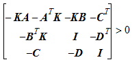
Nexxim Simulator > S-Parameter Technical NotesReference Nodes on S-Parameter ElementsWhen an S-parameter element is inserted in the schematic, the dialog allows you to specify a reference node (see Creating an N-Port Model in the Schematic Editor topic.) The two choices are Implied reference to ground and Common reference pin. When implied reference to ground is selected, or when Common reference pin is chosen and then connected or shorted directly to ground in the schematic, Nexxim does not make any adjustments to the S-parameter matrix. When a Common reference pin is unconnected or is connected to ground through a resistor, Nexxim uses matrix operations to adjust the S-parameters. When a Common reference pin is left unconnected, Nexxim connects the pin to ground through a resistor with value 1012 ohms. The formulas below are for the frequency domain at a single frequency. It is convenient to convert from S-parameters to the equivalent Z parameters. The Z-matrix takes the vector of input currents into the vector of terminal voltages: V = Z * I. Suppose that the S-parameters all have a common reference impedance Zref and that the resistor inserted between the reference node of the S-parameter block and ground is of value R>0. Let matrix A be the 2x2 matrix with the value R/Zref in each of the four locations. Then the effective Z-matrix of the structure with the resistor Zeff = Z + A. Put in the form of matrix manipulations for the S-parameters:
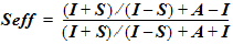
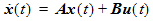
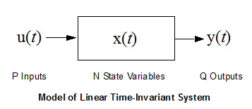
where I is the 2x2 identity matrix. State-Space MethodS-parameters describe a system in terms of its frequency-dependent responses. Nexxim’s state-space model assumes a linear time-invariant (LTI) system with a vector of inputs u(t) of length P and a vector of outputs y(t) of length Q:
The state-space model represents the data as a vector of N state variables x(t) representing the responses of the system for all inputs in the specified range, and four state-space matrices, A, B, C, and D. See State Space References [1] in S-Parameter References for an introduction to state space modeling. State Equations and Output EquationsThe vector of state equations:
where:
gives the rate of change of the state variables (responses), computed as a weighted sum of the current state vector and the input vector. Matrix A, the state matrix, contains the frequency-dependent poles of the system. Matrix A has dimension N by N. Matrix B, the input matrix, contains the weights applied to the input vector. Matrix B has dimension P by N. From the time derivatives of the state variables x(t) one may calculate the values of x(t + Dt) using the vector of output equations:
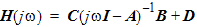
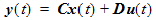
The output vector is a weighted sum of the current state vector and the input vector. Matrix C, the output matrix, contains the weights applied to the state vector. Matrix C has dimension Q by N. Matrix D, the feedforward matrix, contains weights applied to the input vector. Matrix D has dimensions Q by P. Transfer FunctionThe transfer function is the ratio of the output to the input. In Laplace space s, the transfer function can be expressed in terms of the state space matrices:
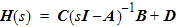
where sI is an N by N matrix with s on the diagonal and zeros elsewhere. H(s) is a matrix of frequency-dependent transfer functions with dimension Q by P, one output for every input. Impulse Response and StabilityThe impulse response h(t) is the response of the system to the delta function, a pulse of vanishingly narrow width. The impulse response is the inverse Lagrangian of the transfer function, and can be expressed in terms of the poles of the system pi (the entries of matrix A).
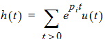
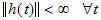
Bounded-In, Bounded-Out (BIBO) stability specifies that as long as the input is bounded, the output must be bounded. For BIBO stability, the exponential factor ept must decay rather than increase. Thus, all the poles pi must have negative real parts. For BIBO stability, the norm of the impulse response must always be finite:
State Space Fitting MethodsBy default, Nexxim uses an Ansoft-proprietary fitting method, the Tsuk-White Algorithm (TWA) for calculating the state space matrices. The TWA algorithm for state-space fitting is an alternative to rational fitting. TWA generates the poles of the state-space fit from the singular value decomposition of Loewner matrices derived from the input data [State-Space Reference 2]. Unlike rational fitting, TWA is not an iterative procedure. Thus, TWA can produce high-quality state-space fits in much less time than rational fitting. The TWA algorithm may succeed where rational fitting produces a bad fit or a fit that is good but nonpassive on a problem too big for passivity enforcement. The option: s_element.twa=1|0 can be used to toggle between the TWA algorithm (1) and the rational fitting method (0). Causality Checking and EnforcementThis topic explains how Nexxim handles causality checking and enforcement of S-parameter data. Any physical, realizable system must be causal,
that is, its response cannot precede the excitation that produces the
response. Although causality is a consideration in any physical system,
the focus for signal and power integrity simulations is on linear, time-invariant
(LTI) systems, a category that includes (but is not limited to) interconnects,
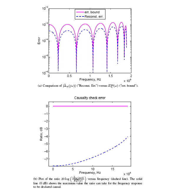
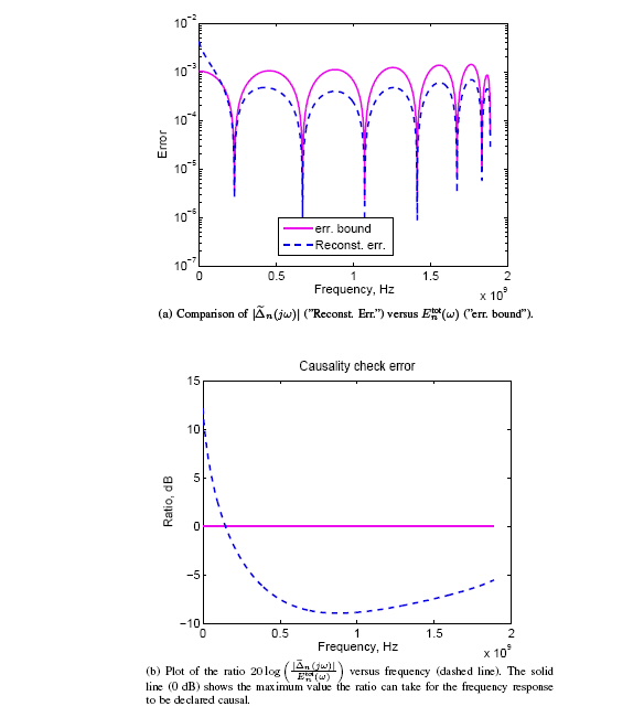
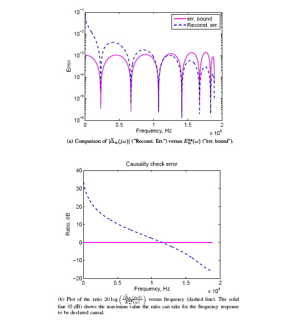
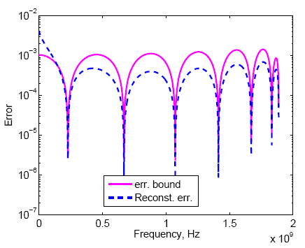
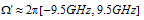
packages, connectors, and board-level systems. Nexxim can check for causality violations, and can correct causality problems. The basic strategy for both checking and correction is to compute a known-causal reconstruction of the data, and then to compare the reconstruction error to a known error bound or threshold for noncausality over all frequencies. In Nexxim the threshold for noncausality is proportional to the overall tolerance for errors in the rational fit. An Example of a Noncausal SystemThe diagram below shows the internal results of the Nexxim causality checker with a transmission line. NOTE: These internally-computed values are not available for plotting in Designer.
The error bound for noncausality is the solid magenta line. The maximum value for the error bound has been set to 2x10⁻³. The reconstruction error is the dashed blue line. At the lowest frequencies, the reconstruction error exceeds the threshold, indicating a causality violation. Nexxim reports the percent error as the difference between the two values, times 100. Symptoms of NoncausalityProblems with causality of frequency response data show up as errors in the accuracy and stability of the simulation. Causality and AccuracyBefore starting transient simulation, Nexxim calculates a causal macromodel that approximates the original data in the frequency domain. If the original data are noncausal, the approximation by the macromodel may not be accurate. The more severe the noncausality, the higher will be the fitting error of the approximation. If the fitting error is greater than 10%, transient analysis will not even begin. Even when transient runs, a fitting error greater than 1% can give results that are inaccurate, often to a degree that is unacceptable. Causality and StabilityThere is a strong correlation between causality issues
and passivity violations. Often, the fitting error is acceptable, but
the macromodel is nonpassive. A passive system does not generate energy;
it can only dissipate or transform energy. In the frequency domain,
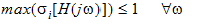
the scattering or S-parameters of passive systems (including macromodels)
have singular values that are less than or equal to 1 at all frequencies
Unstable results can be avoided if the macromodel is passive, or can be made passive. Thus, one possible solution for instability issues is to try passivity enforcement on the macromodel before running transient again. However, passivity enforcement increases the runtime, and the degree of noncausality adds to the problem. To obtain an acceptable fit with noncausal data, the macromodel may require a large model order (number of poles > 200). Model order has a direct effect on the passivity correction runtime. A second, related issue is memory usage. Passivity correction encounters memory problems for systems with large numbers of I/O ports (>200). When the model order is also high due to noncausality, passivity enforcement is at high risk of running out of memory, which will cause transient to terminate without simulating anything. Memory problems during passivity enforcement are common with package models for memory subsystems. In addition, passivity enforcement affects the accuracy of the result. If the calculated passive macromodel has a fitting error (to the original data) of more than 10%, transient simulation will not begin. The higher the nonpassivity (as measured by the maximum singular value), the greater chance that the macromodel will be inaccurate. Hence, strong causality problems typically lead to poorly-fitting passivity-enforced macromodels. Many companies now require that all frequency-response data coming from commercial field solvers be certified to be causal. Sources of NoncausalityTouchstone data come from three different sources: from measurements, from field solvers (2-D, 3-D, or 2.5-D), and from circuit solvers. Any of these sources can introduce noncausality into data. This tech note analyzes causality issues in data from field solvers and circuit solvers. Causality Issues with Field SolversThere are many sources of noncausality in data from field solvers. • Constant loss-tangent models for modeling frequency-dependent dielectric behavior often contributed to noncausality in the data. Fortunately, the Debye and Djordevic-Sarkar models for dielectric constants have eliminated this source of noncausality. • Subsystems in field solvers can have noncausal models. • Discontinuity of the field solutions can produce noncausal data. • Noncausal interpolating functions during interpolation sweep are a frequent source of problems. • Large inaccuracies in the discrete sweep solution at a frequency can also introduce noncausality. Causality Issues with Circuit SolversCircuit solvers, too, can introduce noncausality into
Touchstone data. Most of the noncausality comes from components meant
to work at radio or microwave frequencies. A typical example of such
a component is the transmission line model (e.g., coaxial cable). The
dielectric loss of the lines is still modeled by constant loss-tangent
models (conductance is made to vary linearly with frequency, while capacitance
is held constant), and the conductor loss by Testing for CausalityCausality imposes constraints on the impulse response and the frequency response of an LTI system. The constraints are the basis for causality checking the S-parameter data for an LTI system read from a Touchstone file. Causality Constraints on the Impulse ResponseConsider a system with impulse response h(t) that is excited by a signal x(t), producing an output y(t). For an LTI system, these quantities are related through the convolution integral:
(1) where the operator (*) denotes a linear convolution. A causal system must be nonanticipatory, that is, y(t) from equation (1) should
depend on x(t) for
(2)
By equation (2), a causal h(t) is sufficient to ensure that y(t) does not precede x(t). It can be shown that a causal h(t) is both necessary and sufficient. Causality Constraints on the Frequency ResponseThe frequency-domain response H(jw) is the Fourier transform of time-domain signal h(t):
(3)
where F{} denotes the Fourier transform, j2 = -1, and w is the angular frequency. The constraints on a causal frequency response can be derived as follows. A causal h(t) satisfies the condition:
(4)
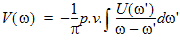
where the function sign(t) returns 1 for t>0, 0 for t=0, and -1 for t<0. Taking the Fourier transform of equation (4), we obtain:
(5)
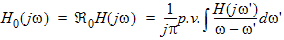
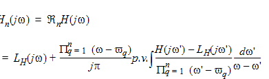
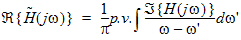
where F{} denotes the Fourier transform, and the integral is defined according to the Cauchy’s principal value (p.v.). The right-hand side (RHS) of equation (5) is known as the Hilbert transform of H(jw). The Hilbert Transform Test for CausalityThe frequency response H(jw) can be separated into its real and imaginary parts:
(6)
From equation (6), the real and imaginary parts of a causal H(jw) are Hilbert transforms of each other. If a frequency response satisfies this constraint, it is declared causal. Let R0 denote the operator in the RHS of (5):
(7)
Then from equation (5) a causal frequency response maps onto itself:
(8)
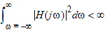
The Generalized Hilbert Transform Test for CausalityThe conditions in (6) are sufficient for causality, but are not necessary. In particular, the constraints in (6) are true only for a response H(jw) that is square-integrable. The function H(jw) is square-integrable if:
(9)
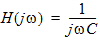
The constraints in (6) have been shown to be necessary and sufficient conditions for causality with square-integrable functions (see Causality Reference [3]). An example of a square-integrable function is the driving-point impedance of a parallel RC circuit:
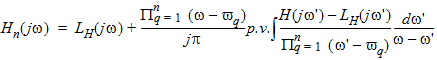
where G=1/R and C are positive real constants. Here are example functions that are are not square-integrable (R, L, and C are positive real constants). These functions are causal but do not satisfy (6): 1. 2. 3. 4. Any linear combination of 1, 2, and 3. For functions that are not square-integrable, the necessary and sufficient conditions for causality are given by the generalized Hilbert transform (see Causality Reference [3]). The generalized Hilbert transform of H(jw), Hn(jw), is given by:
(10)
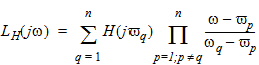
where n is the number of subtraction points, and

represents the subtraction points spread over the available bandwidth W (see Testing for Causality of Touchstone Data for details on W), and LH(jw) is the Lagrangian interpolation polynomial for H(jw) (see Causality Reference [6]):
(11)
The Hilbert transform is a special case of the Generalized Hilbert transform when n=0, hence the term “Generalized.” From equations (10) and (11), if n = 0 then LH(jw) = 0, and the P terms in (10) disappear. The resulting equation is the Hilbert transform of H(jw), equation (8). Let Rn denote the reconstruction operator in the RHS of (10):
(12)
Then a causal frequency response, square-integrable or not, maps onto itself under Rn:
(13)
Equation (13) can be used to test whether or not a frequency response is causal. A causal frequency response will map onto itself under the operator Rn, but a noncausal response will not. A further constraint on a causal frequency response is that all its network transforms must also be causal. That is, if H(jw) is a scattering parameter and is causal, then the corresponding impedance and admittance parameter must also be causal. Truncation and Discretization Errors in Causality TestingCausality of a frequency response can be tested by verifying
whether or not the frequency response satisfies (13): a causal response
will map onto itself if the operator Rn
is applied. On the other hand, if the frequency response is noncausal,
then it will not map onto itself and hence will not satisfy (13). However,
the test in (13) is valid only when H(jw) is known continuously for
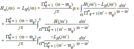
all frequencies One possibility to check for the causality of Touchstone data is to use the test in (13), but limit the integral in (12) to W, ignoring the contributions of the out-of-band integral, and interpolate H(jw) within W, so that (12) can be computed. However, the results of this new test are not reliable, due to two sources of error. Error introduced by ignoring the out-of-band contribution is called the truncation error. Errors introduced when approximating a continuous response from data at discrete frequencies is called the discretization error. The unreliability that results from these two errors can lead one to falsely declare a causal response as noncausal (false positive) or a noncausal response as causal (false negative). Such false detections should be avoided. Therefore, for tabulated data, a modified test based on (13) that is also reliable is needed. Since truncation and discretization errors are the sources of unreliability, the modified test has to account for both. Accounting for the Truncation ErrorTo compensate for the missing out-of-band data, the following formulas can be applied. Separating (12) into in-band and out-of-band contributions, we obtain:
(14)
In (14), the integration term in WC
is the out-of-band contribution to H(jw). The Cauchy’s integral
in this term can be replaced by a regular integral, since the integrand
does not have a singularity for We can separate the modified integral to reflect the separate contributions from H(jw) and LH(jw), respectively:
(15)
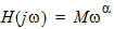
The integration term for LH(jw) can be abbreviated as Cn(jw). Since LH is an nth-order polynomial, a closed-form expression for Cn(jw) can be derived. The integration term for H(jw) can be abbreviated as -En(jw). This is the truncation error. Since H(jw) is not defined outside W, En(jw) cannot be evaluated directly. However, the error introduced by omitting this term can be quantified by fixing the behavior of H(jw) in WC. If:
(16)
where M is a real constant,
(17)
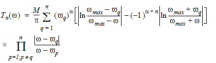
where Tn is the truncation error bound:
(18)
The bound in (18) has been shown to be tight (see Causality Reference [5]). This bound can be made small by increasing the number of subtraction points, n. Due to its Lagrange-polynomial nature, Tn(w)
is bounded only for frequencies
(19)
and where e
is a small number (<0.1). It can be seen from (18) that Tn(w) decreases
as n increases. From (17), when Tn(w) is reduced, so is The best approximation to Hn(jw),
(20)
Accounting for the Discretization ErrorNext, we consider how to evaluate the in-band contribution,
the second term in (20). Since the functional form of H(jw) is
not known in W,
this integration cannot be evaluated analytically. Since the integrand
is singular for w’
= w, numerical
integration will not be robust unless the integrand is regularized.
Simple integration methods such as the Trapezoidal rule and Simpson’s
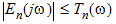
method can be employed. If
(21)
The bound for the discretization error is obtained
by subtracting the estimates
(22)
where n1 and n2
are two different integration rules. In Nexxim, the two rules are Simpson’s
method and the Trapezoidal rule, respectively.The discretization error
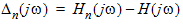
The Causality Test with Minimized ErrorsNow we can construct a causality test that minimizes
both truncation and discretization errors. Let
(23)
(24)
Then
(25)
Therefore, the reconstruction error
(26)
If and only if H(jw) is causal, the error Let
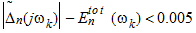
(27)
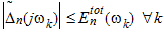
Thus for a causal signal, the reconstruction error never exceeds the total error bound::
(28)
When this condition is met, any causality violations in H(jw) are too small to be flagged, and the data are declared causal.
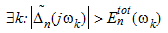
If, on the other hand, the reconstruction error exceeds the threshold at any frequency:
(29)
then H(jw) is declared to be noncausal. Nexxim reports the causality as a percent error:
Fixing the Values for The Total Error Bound
|
Note |
The HSPICE S-Model parameter DELAYHANDLE=1 has the same effect as option convolution =1. |
• convolution=2: The impulse response is a train of impulses in the time domain, given by the inverse Fast Fourier Transform. This setting yields an impulse response that is accurate in-band and usually passive. However, the transient waveforms may have discontinuity effects.
• convolution=3: The impulse response is the linear interpolation of the inverse FFT results. This setting yields an impulse response with a low probability of passivity violations, but there is significant filtering towards the top of the frequency range of the input data.
The convolution=1, 2, 3 options apply the convolution method globally to all S-parameter models in the design. The convolution option can be overridden in a particular model by setting model parameter CONVOLUTION. The setting of a CONVOLUTION model parameter overrides the global option convolution setting for S-element instances that reference the given model.


HFSS视频教程 ADS视频教程 CST视频教程 Ansoft Designer 中文教程
|
Copyright © 2006 - 2013 微波EDA网, All Rights Reserved 业务联系:mweda@163.com |
|

 . When a macromodel
is nonpassive (maximum singular value >1.00), there is a potential
for instability, with unbounded values for node voltages and branch
currents. Terminations that do not match the input impedance increase
the probability of instability, even with modest nonpassivity.
. When a macromodel
is nonpassive (maximum singular value >1.00), there is a potential
for instability, with unbounded values for node voltages and branch
currents. Terminations that do not match the input impedance increase
the probability of instability, even with modest nonpassivity. variations, while making the inductance
constant with frequency.
variations, while making the inductance
constant with frequency.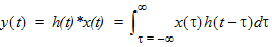


 .
Frequency responses in the form of Touchstone data are known only at
discrete frequencies in the bandwidth
.
Frequency responses in the form of Touchstone data are known only at
discrete frequencies in the bandwidth 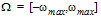 , where
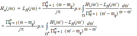
 .
.
 ,
, 
 , where:
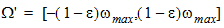
 , the truncation error.
Thus, the disadvantage of not knowing the frequency response outside
of the bandwidth (i.e., in
, the truncation error.
Thus, the disadvantage of not knowing the frequency response outside
of the bandwidth (i.e., in  , is obtained by ignoring the
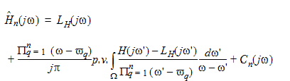
 is the numerical approximation to
  , then the error in this approximation,
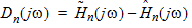
 computed using two different integration rules, and is
given by:
computed using two different integration rules, and is
given by: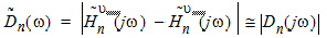
 is reduced if
the bound
is reduced if
the bound  is reduced.
The bound
is reduced.
The bound  is reduced
by decreasing the frequency step in the tabulated frequencies.
is reduced
by decreasing the frequency step in the tabulated frequencies. denote the numerical reconstruction error
and
denote the numerical reconstruction error
and the ideal reconstruction
error:
the ideal reconstruction
error: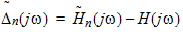
 can be shown to be:
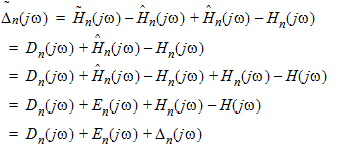
 satisfies the following
inequality for any
satisfies the following
inequality for any 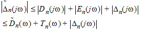
 vanishes at all frequencies.
 be the total error bound, the sum of the discretization and truncation
error bounds
be the total error bound, the sum of the discretization and truncation
error bounds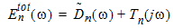

 must
also vary with n. Also, since
must
also vary with n. Also, since  varies with frequency step,
  must vary with frequency step as well. It
is important to set
must vary with frequency step as well. It
is important to set  to
reasonable values. Very large values for
to
reasonable values. Very large values for  can hide causality violations, while very
small values can flag any response as noncausal.
can hide causality violations, while very
small values can flag any response as noncausal. . Typically, the
maximum tolerable magnitude of noncausality,
. Typically, the
maximum tolerable magnitude of noncausality,  , is known a priori. In previous versions,
Nexxim set
, is known a priori. In previous versions,
Nexxim set  to
10
to
10 is tied by default
to the tolerance for the fitting error,
is tied by default
to the tolerance for the fitting error,  . These tolerances are linearly related:
 .
Now, a reasonable value for
.
Now, a reasonable value for  to 0.01 (1%) for S-parameters. To keep
  greater than 0.0001,
 .
In Nexxim,
.
In Nexxim,  is set by the user (with the option causality_check_tolerance),
that value is used and the relationship in equation (30) is not considered.
is set by the user (with the option causality_check_tolerance),
that value is used and the relationship in equation (30) is not considered. has been determined,
a reasonable n is chosen such that the truncation error is always
less than the tolerance by a fixed proportion:
has been determined,
a reasonable n is chosen such that the truncation error is always
less than the tolerance by a fixed proportion:
 , given by:
 .
Based on experimentation, Nexxim sets
.
Based on experimentation, Nexxim sets  is much smaller than
 , the total bound
  follows
 . If the frequency
steps in the tabulated data are not small,
. If the frequency
steps in the tabulated data are not small,  can be comparable in magnitude to
  can
be greater than
can
be greater than  .
When this condition is detected, the best solution is to reduce the
maximum frequency step in the tabulated data and repeat the causality
test until
.
When this condition is detected, the best solution is to reduce the
maximum frequency step in the tabulated data and repeat the causality
test until  satisfies
(33).
satisfies
(33).
 at all frequencies,
the causality test can be run. However, a reliability issue now emerges.
When calculated by equation (22),
at all frequencies,
the causality test can be run. However, a reliability issue now emerges.
When calculated by equation (22),  is not strictly an upper bound. As a result, the condition
in (28) can be met, flagging the response as noncausal, although the
frequency response is really causal. This problem of false positives
can be overcome by computing
is not strictly an upper bound. As a result, the condition
in (28) can be met, flagging the response as noncausal, although the
frequency response is really causal. This problem of false positives
can be overcome by computing  as a strict upper bound, making use of upper bounds for
the integration error in Simpson’s method and the Trapezoidal
rule. However, the resulting bounds have been found to be unreliable
at times.
as a strict upper bound, making use of upper bounds for
the integration error in Simpson’s method and the Trapezoidal
rule. However, the resulting bounds have been found to be unreliable
at times.  using equation (22).
Nexxim uses a heuristic to differentiate between a false positive due
to
using equation (22).
Nexxim uses a heuristic to differentiate between a false positive due
to  and a genuine
noncausality. A false positive due to
and a genuine
noncausality. A false positive due to  usually results in a minor causality violation, while
a genuine positive results in a strong causality violation. Nexxim
considers any violation less than 0.5% to be a minor violation.
A causality violation is computed at
usually results in a minor causality violation, while
a genuine positive results in a strong causality violation. Nexxim
considers any violation less than 0.5% to be a minor violation.
A causality violation is computed at 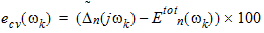
 ,
then a false positive is most likely, and the frequency response is
certified to be causal. If on the other hand
,
then a false positive is most likely, and the frequency response is
certified to be causal. If on the other hand  , the frequency response is declared to be
noncausal. With any kind of violation, Nexxim prints the
, the frequency response is declared to be
noncausal. With any kind of violation, Nexxim prints the  to the console for each
entry in the S-matrix.
to the console for each
entry in the S-matrix.
 , the maximum
magnitude of error that still satisfies the causality checker. Nexxim
sets the default tolerance to be a fraction of the overall tolerance
for fitting errors.
, the maximum
magnitude of error that still satisfies the causality checker. Nexxim
sets the default tolerance to be a fraction of the overall tolerance
for fitting errors.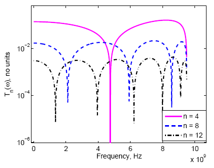
 .
Since
.
Since 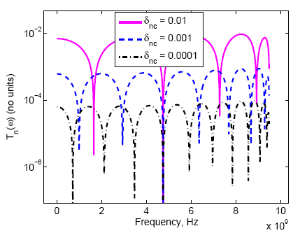

 for
for  .
. . The causality checker tolerance
  . Therefore,
  satisfies (33).
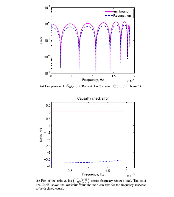
  is compared against
  . From the figure, it is clear that
  is smaller than
  for all frequencies in
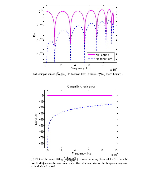
 and
and  .
Let the inductance
.
Let the inductance  , and let
  . Refer to Figure 5.
The simulation parameters are the same as Case 1, except that
. Refer to Figure 5.
The simulation parameters are the same as Case 1, except that  and
and  and
and  . Refer to
Figure 7. The parameters are the same as in Case 1, except that both
. Refer to
Figure 7. The parameters are the same as in Case 1, except that both