|
微波射频仿真设计 |
|
|
微波射频仿真设计 |
|
| 首页 >> Ansoft Designer >> Ansoft Designer在线帮助文档 |
|
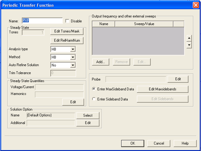
Nexxim Simulator > Running Periodic Transfer Function Analysis from the Schematic EditorPeriodic transfer function (PXF) analysis computes the small-signal transfer function from selected voltage and current sources in the circuit to a specified single output at a frequency that can be swept. A steady-state HB or OSC analysis first computes the periodic or quasi-periodic operating point, on which the small-signal PXF analysis is calculated. In Nexxim, PXF analysis is an extension of the time-varying noise analysis. To run a periodic transfer function analysis on a Nexxim schematic design, perform the following steps: 1. Right-click on the Analysis menu in the Project window to open a menu. 2. Select Add Nexxim Solution Setup from the menu, then slide the cursor to select Periodic transfer Function (PXF) from the subordinate menu. 3. The Periodic Transfer Function solution setup dialog opens:
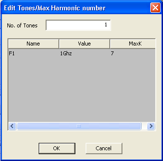
4. Type an Analysis Name (or accept the default name, for example “PXF”). 5. For most simulations, leave the Disable box unselected (the default setting). Selecting this box lets you store multiple solution setups for later use. (Note that if a solution setup is disabled before the analysis is run, any changes made to the design will invalidate the simulation results.) 6. In the Steady State panel, click the Edit Tones/Maxk button. The Edit Tones/Max Harmonic Number dialog opens:
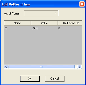
• Enter the number of tones to be used in the steady-state phase of the analysis. The tones are listed with names F1 ... Fn. These names cannot be changed. • Click on a Value field in the row for one of the tones to enter the frequency for the steady-state analysis for that tone. • Click on a MaxK field in the row for one of the tones to enter the Max. Harmonic Number for the steady-state analysis for that tone. • Click OK to close the Edit Tones/Maxk dialog and return to the Periodic Transfer Function dialog. The Number of tones field now shows the number of tones you specified in the dialog. 7. Optionally, click on the Edit RelHarmNum button to open the corresponding dialog:
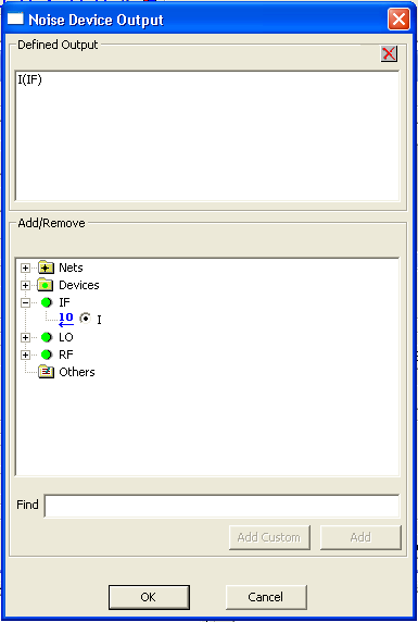
• The No. of tones, Name, and Value fields reflect the settings from the Edit Tones/Maxk dialog. The number, name, and value of tones cannot be changed in the Edit RelHarmNum dialog. Click OK to return to the Periodic Transfer Function dialog box. • Click in the RelHarmNum field for a frequency to set the relative harmonic number offset for that tone. Refer to the TV Noise Technical Notes topic for information on the use of the RelHarmNum offsets. Click OK to return to the Periodic Transfer Function dialog box. 8. Select the Analysis type from the pulldown. The default is harmonic balance (HB). You can choose oscillator analysis (OSC) instead. • When HB is the Analysis type and one-tone analysis has been specified in the Edit Tones/Maxk dialog, the Method field is activated. Use this field to select HB or shooting (HB is the default). See Handling Strongly Nonlinear Circuits in the HB topic for details on the Method entry. • When HB is the Analysis type, the Auto Refine Solution field is activated. Use this field to select Yes or No (No is the default). See Increasing Accuracy or Speed in the HB topic for details on the Auto Refine Solution entry. • When HB is the Analysis type and more than two tones have been specified in the Edit Tones/Maxk dialog, the Trim Tolerance field is activated. Use this field to set a tolerance value. See Increasing Accuracy or Speed in the HB topic for details on the Trim Tolerance entry. 9. Optionally, click the Edit button at the lower right of the Steady State Quantities panel to add voltages, currents, and harmonic outputs from the underlying analysis (HB or OSC). These additional output quantities are available in the Report dialog after simulation has been performed. Expand the Nets and devices icons to display lists of the available quantities. To have Nexxim calculate outputs from the steady state analysis step, use the checkboxes to select the outputs. Expand the Harmonics icon to display a list of the available harmonics. To specify particular harmonics for Nexxim to use when calculating outputs from the steady state analysis step, use the checkboxes to select the harmonics. If you do not select any harmonics, harmonics DC, F1, 2F1, 3F, and 4F1 are automatically selected. In the Report dialog, only selected harmonics are available for plotting. Click OK to return to the Periodic Transfer Function dialog box. 10. The underlying TV Noise analysis requires a sweep of output frequencies. Click Add in the Output frequency and other sweeps field. The Add/Edit Sweep dialog opens. • Make sure F (frequency) is the entry in the Variable field. • Use the radio buttons to select one of the following: Single value, Linear step, Linear count, Decade count, or Octave count. • Type the sweep values into the Value text box (for Single value), or into the Start, Stop, and Step text boxes (for Linear, Decade, or Octave count), and make sure that the appropriate units are selected for each. • Click Add, and then click OK to close the dialog box. • The Periodic Transfer Function dialog box reappears. The sweep definition appears in the Output frequency and other sweeps field. (The Output frequency and other sweeps display includes fields labeled Offset of F1 and Sync. These fields are not used by Nexxim PXF analysis.) 11. Click on the Edit button next to the Probe field to open the Noise Device Output dialog.
Expand the Nets and Devices icons to display lists of the available quantities. Click in the checkbox for the single output to be used in the PXF analysis. Click OK to return to the Periodic Transfer Function dialog box. 12. If you have specified a single frequency in the Steady State Tones field, use the radio buttons to select either Enter MaxSideband Data or Enter Sideband Data. See the TV Noise Theory of Operation topic for more information. • To enter a maximum sideband to use in calculating the input frequencies, select Enter MaxSideband Data and click Edit Maxsidebands. Click in the MaxSidebands field at the right and enter the number of sidebands to use. (The Name and Value fields reflect your selection in the Steady State Tones field, and cannot be changed in the Edit MaxSidebands dialog). Click OK to return to the Periodic Transfer Function dialog. • To enter specific sidebands to use, select Enter Sideband Data and click Edit Sidebands. Enter the first sideband value, then press the Add Row button to open another line in the dialog. To delete a row, select it and press the Delete Row button. When you have finished entering sidebands, click OK to return to the Periodic Transfer Function dialog. 13. If you have specified multiple frequencies in the Steady State Tones field, only the radio Enter Sideband Data button is active. See the TV Noise Technical Notes topic for more information on the use of the Sideband Data entries. • To enter specific sidebands to use, click Edit Sidebands. Enter the first set of sideband values (one value per frequency), then press the Return or Tab key o open another line in the dialog. When you have finished entering sidebands, click OK to return to the Periodic Transfer Function dialog. 14. Optionally, use the fields in the Solution Option panel to add analysis options and other Nexxim options to the design. • Click the Select button on the Name field to open the Select Solutions dialog. On the Select Solutions dialog, click New. The Solution Options dialog box appears. Use the Name field to name the new option settings. Select the HB Options or OSC Options tab, depending on the selection for the Underlying analysis type made earlier (Step 8). Make the appropriate changes to option values, then click OK to return to the Select Solutions dialog box. On the Select Solutions dialog, click the name of the new option settings, then click OK to return to the Periodic Transfer Function dialog. The name of the new option settings appears in the Name field of the Solution Option panel. • Click the Edit button on the Additional field to open a text-entry dialog, Edit additional options. Use the text box to enter any Nexxim options exactly as they are to appear in the netlist. Click OK to return to the Periodic Transfer Function dialog. 15. Click Finish to close the Periodic Transfer Function dialog. The solution setup is added to the Project tree under the Analysis icon. 16. Run the simulation: • Expand the Analysis icon on the Project tree, click on the desired solution setup, and select Analyze from the menu. If the circuit is set up correctly, the analysis begins immediately and a red progress bar appears. • The Message Window signals success or failure. • For details on creating and modifying reports, see Generating Reports and Postprocessing.
HFSS视频教程 ADS视频教程 CST视频教程 Ansoft Designer 中文教程 |
|
Copyright © 2006 - 2013 微波EDA网, All Rights Reserved 业务联系:mweda@163.com |
|