|
微波射频仿真设计 |
|
|
微波射频仿真设计 |
|
| 首页 >> Ansoft Designer >> Ansoft Designer在线帮助文档 |
|
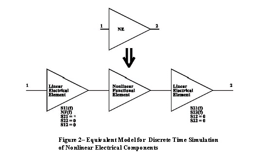
Nexxim Simulator > Discrete Time Simulation of Nonlinear Behavioral ComponentsThe nonlinear discrete time simulation technique described here is used for processing bandpass modulated signals through nonlinear behavioral components (e.g., amplifiers, mixers, frequency multipliers). Generally, nonlinear behavioral components are not only power dependent, but also frequency and/or temperature dependent. An equivalent model is used for nonlinear components in discrete time simulation to separate the power dependent characteristics from frequency and temperature dependent characteristics. All nonlinear behavioral two-port components are assumed unidirectional (i.e., S12 = 0). Each nonlinear component is partitioned into three segments: a linear electrical (active) input component, a nonlinear functional component, and a linear electrical (passive and noiseless) output component. This arrangement is shown in Figure 2 below.
In this model, the power dependent characteristics of S11, S12 and S22 are ignored. The frequency and temperature dependent small signal S11 and NF are associated with the input linear electrical component. The power dependent characteristics of S21 are associated with the nonlinear functional component. The frequency and temperature dependent small signal S21 and S22 are associated with the output linear electrical component. For discrete time simulation, the linear electrical input and output components are associated with other connected linear electrical components and simulated as a linear electrical sub-design as discussed in the previous section. The nonlinear characteristic of a two-port component in Designer is described by its nonlinear figures-of-merit or nonlinear measured data. Only the nonlinear characteristic of S21 is considered in discrete time analysis techniques even though S11, S12 and S22 may possibly be power dependent too.
Modeling Nonlinearity with Polynomial Power Series It is always assumed that nonlinear measurements are
obtained when the input and output ports of the nonlinear component
are terminated in 50Ω. Nonlinear measurements
of a two-port component typically include the AM-AM and AM-PM effects.
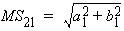
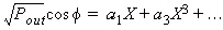
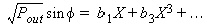
This nonlinear relationship between S21 and P1
(the available input power) or, equivalently, between Pout
and P1
is represented by the following power series polynomials:
The coefficients a1, a3, a5,... and b1, b3, b5,... are calculated using a least-squares curve fitting technique based on the user-supplied measurements P1 - Pout data or P1 - S-parameters data. For example, a set of coefficients can be obtained based on the following power amplifier P1 - Pout measured data (in 50ohm terminations). RTH_PA 2-port POUT dBm P1 dBm, FREQ = 900MHz
If the user chooses to provide the nonlinear figures-of-merit (OIP3 or P1dB and Psat) instead of measurement data, the power series coefficients are approximated by 
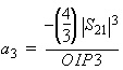
ai = 0, i = 5,7, ... bi = 0, i = 1,3,5, ... where: S21 is the linear small signal gain OIP3 is the output power at the third order intercept point. In this case, the simulations tend to be less accurate. Calculating a Nonlinear Output Voltage Assuming a bandpass modulated input signal of the form: 
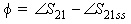
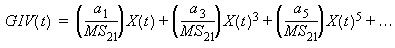
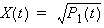
where Vs(t) is the baseband input voltage  is the phase of the input modulated signal 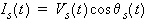 = In-phase envelope of the input signal 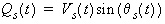 = Quadrature-phase envelope of the input signal  , where fc is the carrier frequency. The nonlinear output voltage is calculated as: 
where: 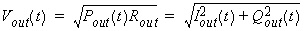
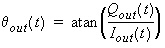


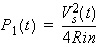
with 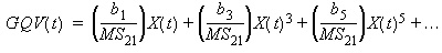 and
HFSS视频教程 ADS视频教程 CST视频教程 Ansoft Designer 中文教程 |
|
Copyright © 2006 - 2013 微波EDA网, All Rights Reserved 业务联系:mweda@163.com |
|
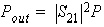 = the output load power (assuming RL = 50Ω)