关于主从边界条件看色散曲线的问题

Model Setup
[backcolor= transparent]First we must configure HFSS to use its eigenmode solver; HFSS>Solution Type...>Eigenmode. Next, the unit-cell of parallel plate waveguide has to bedrawn in HFSS. It consists of rectangular substrate asshown in Fig. 1. The dimensions of the unit-cell are 5.0x5.0x2.54 mm³ andthe substrate material is Rogers RT/duroid 6010/6010LM.
[backcolor= transparent]

[backcolor= transparent]
Periodic Boundary Conditions
[backcolor= transparent]1. Select the negative y-z face of the unit-cell and assigna Master Boundary Condition (mx); you have to define the UVector which starts at (-2.5, -2.5, 0) and ends at (-2.5, 2.5,0). Thecompleted boundary assignment should look like Fig. 3. Next select the positivey-z face of the unit-cell and assign a Slave Boundary Condition (sx).Again define the U Vector which starts at (2.5, -2.5, 0) and ends at(2.5, 2.5, 0). Then input the phase delay using a variable (px) as shownin Fig. 4 and input an initial value (90 deg) as shown in Fig. 5. *Do not forgetto put in “deg.”
[backcolor= transparent]

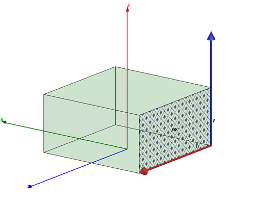
Figure 3. Completed master boundary condition.

[backcolor= transparent]

Figure 4. Phase delay.

[backcolor= transparent]

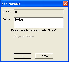
Figure 5. Variable setup.

[backcolor= transparent]

2. Do the same to the x-z faces of the unit-cell. Label themaster as my and the slave as sy. For sy make sure toreverse the V Vector and use a variable (py) and input an initialvalue (0 deg). *Do not forget to put in “deg.”

[backcolor= transparent]
Analysis/Optometrics Setup
[backcolor= transparent]Before the eigenmode analysis can be started, several steps need to be completedfirst. First, add a solution setup and input the values as depicted in Fig. 6. In addition, in theoptions tab of the Solutions Setup, input a minimum converged passes of3.
[backcolor= transparent]

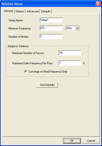
Figure 6. Solution setup dialog.

[backcolor= transparent]Next, parametric sweeps need to be added. So chose HFSS>OptometricsAnalysis>Add Parametric. You will need to do this three times for each ofthe high-symmetry points of the Brillouin zone.
[backcolor= transparent]

For the first parametric sweep, we will go from Г toХ and this will be labeled 1_Gamma2X. Add a linear step sweep for thevariable px from 15 deg to 180 deg with 15 deg steps. In the Options tabmake sure to check both Save Fields and Mesh and Copy geometricallyequivalent meshes.

[backcolor= transparent]

For the second parametric sweep, we will go from Хto M and this will be labeled 2_X2M. Add a linear step sweep for thevariable py from 15 deg to 180 deg with 15 deg steps. We have to set px to 180 deg. To do this go to General tab and check override for px and input 180 deg as shown in Fig. 7.  In the options tab make sure to checkboth Save Fields and Mesh and Copy geometrically equivalent meshes.

[backcolor= transparent]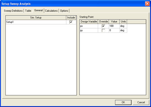

Figure 7. Override px variable.

[backcolor= transparent]

For the third parametric sweep, we will go from M toГ and this will be labeled 3_M2Gamma. Add a linear step sweep for thevariable px from 15 deg to 180 deg with 15 deg steps and also for thevariable py. Select both of these sweeps and Sync them as shown in Fig.8. In the options tab make sure to check both Save Fields and Mesh and Copy geometrically equivalent meshes.

[backcolor= transparent]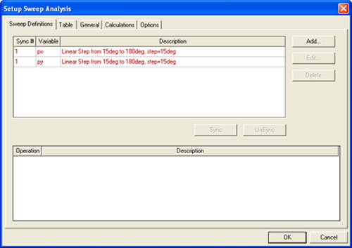

Figure 8. Sync up sweeps.

[backcolor= transparent]
Plotting Results
[backcolor= transparent]

Plots for each parametric sweep have to be made. For the Г to Х parametric sweep, create a report and use the default values (EigenmodeParameters, Rectangular Plot). In the Sweep tab, choose Sweep Design andProject variable values and choose px values from 15 deg to 180 degand for py select only 0 deg. For the Y tab, choose EigenModes>Mode(1)>re. We only wish to look at the real part of the eigenmode, theimaginary part is due to loss which is ignored since a parallel platewaveguide’s loss is negligible for the fundamental mode. The finished plotshould look like Fig. 9.

[backcolor= transparent]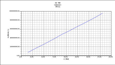

Figure 9. Plot of Г to Х.

[backcolor= transparent]

To plot the X to M parametric sweep, do thesame as for the Г to Х parametric sweep report. However, make py as the primary sweep and set px to 180 deg. The finished plotshould look like Fig. 10.

[backcolor= transparent]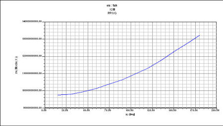

Figure 10. Plot of Х to M.

网上的经典例子，一步步做下来，最后看不到结果。
Plots for each parametric sweep have to be made. For the Г to Х parametric sweep, create a report and use the default values (EigenmodeParameters, Rectangular Plot). In the Sweep tab, choose Sweep Design andProject variable values and choose px values from 15 deg to 180 degand for py select only 0 deg. For the Y tab, choose EigenModes>Mode(1)>re.
没有选sweep的地方。是不是中间少了一步啊?请问有大神知道么?

我用的是HFSS 17 ，有影响么

这个文献是哪篇啊 能不能传上来看看