|
微波射频仿真设计 |
|
|
微波射频仿真设计 |
|
| 首页 >> Ansoft Designer >> Ansoft Designer在线帮助文档 |
|
Dynamic Links and Solver On Demand > Adding a Planar EM Dynamic LinkTo create a dynamic link Planar EM subcircuit: 1. Right-click the icon for the schematic design in the Project tree. 2. Select Add Subcircuit from the menu. A subordinate menu opens. 3. Select Add Planar EM Design from the Add Subcircuit subordinate menu. 4. The Layout Editor opens in a new window. Add geometry and pins to create the Planar EM subcircuit. 5. Click on the icon for the top circuit to make its schematic the active window. The Planar EM subcircuit appears in the Schematic Editor. Pins on the Planar EM subcircuit become ports on the subcircuit in the schematic editor. Wire the subcircuit into the main circuit. An icon for the subcircuit appears in the Project tree. Planar EM subcircuits use the default Planar EM simulation setup, unless overridden as described below.
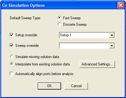
Overriding Subcircuit Setup During Cosimulation with Planar EM You can modify the auto-generated subcircuit simulation setup for cosimulation with Planar EM. Create a setup and a sweep in Planar EM, then invoke the Cosimulation options dialog:  This will setup the Planar EM subcircuit to always use the specified setup/sweep at cosimulation time.
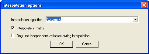
Clicking Advanced Settings when Interpolate from existing solution data is selected, opens the Interpolation options dialog.  Click the down arrow in the Interpolation algorithm dialog to display the following interpolation algorithm options: Automatic – Linear interpolation is used even if the grid is not full, in which case required grid points that are missing are computed using Inverse Least Squares with Shadowing, no Hyperplanes. Linear – When a full grid of solutions is available, the cube of solutions which surrounds the solution to be interpolated is located. The corners of this cube are linearly averaged to determine the interpolated solution. If a full grid is not available, an error is reported and the interpolation fails. Inverse Least Squares with Shadowing and Hyperplanes – Least squares interpolation with shadowing and hyperplanes. Inverse Least Squares with Shadowing, no Hyperplanes – Least squares interpolation with shadowing, but no hyperplanes. The main differences between Linear interpolation and Inverse Least Squares with Shadowing (ILSS) are: — Linear only works with a full grid of solutions; ILSS works on arbitrary data. — Linear only considers nearest data; ILSS uses data that could possibly be distant, although shadowing mitigates this effect. — Linear is not first-order continuous; ILSS is first-order continuous.
Next, select from the Interpolate Y matrix and independent variables options: Interpolate Y matrix uses the Y matrix as the basis for interpolation. When Interpolate Y matrix is not selected, the S matrix is used as the basis. Interpolate Y matrix is selected by default. Circuit particulars determine which basis (S or Y) will yield better results, and it is not possible to decide a priori which one will work best. Use only independent variables during interpolation suppresses the calculation of dependent variable values during interpolation. HFSS视频教程 ADS视频教程 CST视频教程 Ansoft Designer 中文教程 |
|
Copyright © 2006 - 2013 微波EDA网, All Rights Reserved 业务联系:mweda@163.com |
|