Monitor
 Monitors
  Field Monitor Field Monitor
This dialog box gives you the opportunity to define field monitors
that you might need to obtain additional information on the electromagnetic
field distribution inside your structure. It is possible to define frequency
as well as time monitors. After a calculation, you can observe your field
monitors by selecting them in the .
Labeling frame
Name:
Displays the name for the field monitor either as a user input or automatically
generated.
Automatic labeling:
This check button enables or disables the automatic labeling for the defined
field monitor. The automatically generated label consists of the
selected monitor type, including either the specified frequency or time
sample settings of the frequency or time monitor, respectively.
Type frame
E-Field:
The electric field vectors will be stored.
H-Field and
Surface current: Selecting this monitor creates two monitor entries
in the result tree. The first one shows the magnetic field vectors. The
second one (labeled with "Surface Current") uses the magnetic
fields on the surfaces of "PEC" or "lossy
material" solids to calculate the surface currents there.
Surface current
(TLM only): Just the surface currents will be calculated. Only
supported by TLM Solver.
Powerflow:
This monitor stores the Poynting vector of the
electromagnetic field. The monitor represents the maximum value (peak
value) of the power flow at every spatial point, encountered within one
period of time. Therefore, this type of monitor is time independent.
Current density:
If there are electric losses inside of the calculation domain, the currents
inside of these materials are stored in this type of monitor.
Power loss
density/SAR:
See
SAR calculation overview for detailed information.
Electric energy
density / Magnetic energy density: Choose one of these monitors
if you want to store the electric/magnetic energy density throughout the
monitor volume. These monitors represent the maximum values (peak values)
of the energy density within one period of time. Therefore they are time
independent.
Farfield/RCS:
For RCS calculations use a plane wave excitation. See Farfield Overview for detailed information.
Note:
Farfield monitors must not have two parallel magnetic/electric boundaries&endash;one
of two parallel boundaries must be of the type open (PML).
Field source: This monitor records
the tangential fields on a prescribed box surface. The recorded data can
be used as a near field source for the time domain solver
in other projects.
Note:
The data is saved in the results folder as "name of the source.fsm".
This monitor is available for the time domain and the tetrahedral frequency
domain solvers. It records the data at the specified frequencies. It is
recommended to use the proprietary FSM
nearfield data format in software products of CST. In
order to use the recorded fields outside of CST products it is recommended
to use the NFS
nearfield scan data exchange format. See here
for more details.
Note:
The minimum frequency Fmin is
required to be an integer multiple of the sampling frequency (Fmax
-Fmin) / (Freq.
Samples-1).
Specification frame
Here, the field monitor domain can be specified,
selecting between frequency and time.
Frequency:
The monitor records the chosen field type only for a specific frequency.
If the transient solver is used, this is done by use of a DFT.
Information about a possible normalization can be obtained in the section
Spectral
results from transient solvers.
Frequency:
Enter a valid
to specify the recording frequency of the frequency field monitor. It
should be within the frequency range entered in the Frequency
Range Settings dialog
box, otherwise this monitor will be ignored during the calculation.
Freq.
samples: For field source monitors, you can choose a number of
equidistant frequency samples between Fmin and Fmax where frequency domain
field sources are monitored.
Fmin/Fmax:
This shows the minimum and maximum frequencies available for the monitors.
It can be adjusted for the field source monitors.
Time:
The monitor records the chosen field type at several equidistant time
samples. Note that this feature is not available
for farfield monitors for frequency domain solvers.
Start
time: Enter here the start time for the time monitoring.
Step
width: Enter here the desired step width for the time monitoring.
Together with start and end time this value determines the full number
of recorded time samples. Note that time monitors possibly need a great
amount of disk memory if the step width is chosen too small.
End
time: Selecting this check box offers the possibility to define
a specific endtime for the recording. If it is not selected, the recording
will continue up to the end of the calculation.
Broadband:
If a farfield monitor was selected in the type frame a broadband farfield
can be calculated during the transient solver run. The broadband
farfield monitor is based on an expansion of the farfield in terms of
spherical waves. The origin of the expansion is the center of the bounding
box. It allows to obtain the farfield at any frequency in the specified
range as well as at any time of the simulation. Frequency domain
and time domain results can be accessed by selecting plots of a broadband
farfield monitor and by the plot properties dialog.
Freq.
samples: Choose a number of equidistant frequency samples between
Fmin and Fmax where frequency domain farfields are calculated. Results
for any frequencies in between are interpolated to obtain broadband information.
For a more accurate interpolation over the frequency band increase this
value e.g. to "31". An odd number assures that the result at
mid frequency is not obtained by interpolation.
Accuracy:
Defines the desired accuracy of the farfield. Together with the Fmax and
the size of the structure it determines the number of modes required to
represent the farfield.
Note
that leaving out higher order terms by choosing a lower accuracy is equivalent
to low pass filtering the farfield solution. This saves memory and computation
time. However, the farfield result has usually less detail.
Transient
farfields: This check button activates
the additional calculation of transient farfield information which can
be displayed afterwards for a certain time in the post processing. Note
that in order to accurately obtain time domain farfields the computational
effort is higher than for broadband farfields only.
2D Plane frame
Activate:
Select this check box to define a 2D field monitor
recorded on a specified plane, otherwise the field is recorded considering
the complete calculation domain as a 3D monitor. 2D monitors are only
available for electric or magnetic field type, either as a frequency or
a time monitor.
Orientation:
You can choose the 2D plane normal parallel to any global coordinate axis
X,Y
or Z.
Position:
Enter the position along the chosen direction here.
|
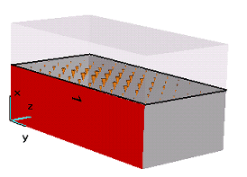
This picture shows a 2D e-field monitor (Normal: X / Position: 0.5 m
(1/2 Xmax) ) of a rectangular waveguide terminated by a electric wall. |
|
Position frame
This frame is only active for field source and
single frequency farfield/RCS monitors.
Use subvolume:
Select this check box to define a subvolume with Xmin, Xmax, Ymin,
Ymax, Zmin,
and Zmax for the field source
monitor. Otherwise, the field is recorded on the boundary of the calculation
domain.
Invert orientation:
Select this check box to record the fields as a source direct inwards.
Otherwise, the fields are recorded for an outward directed source.
Export farfield source
Activates the automatic generation of
a farfield source from the corresponding farfield monitor after a solver
run. All farfield source exports from the same excitation are collected
into a single broadband farfield source file.
OK
Accepts your settings and leaves the dialog
box.
Apply
Accepts your settings without closing the dialog
box so that you can enter another field monitor.
Cancel
Closes this dialog box without performing any
further action.
Help
Shows this help text.
See also
Boundaries, Frequency
Range Settings, Modeler View,
SAR calculation overview,
Farfield Overview, Reference
value and Normalization


HFSS视频教程
ADS视频教程
CST视频教程
Ansoft Designer 中文教程
|
