淘宝官方店推荐课程在线工具联系方式关于我们

	CST视频教程推荐 CST微波工作室入门与应用详解 \| CST使用操作基础

首页 >> CST教程 >> CST2013在线帮助系统

Nonlinear Mechanical Solver Overview

Introduction

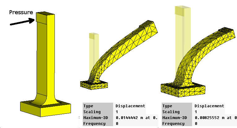
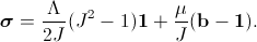
The linear mechanical solver is capable to correctly describe only very small deformations. In contrast, the nonlinear solver is utilized to describe the finite deformations. The difference in the solutions can be seen in the following figure:

The left figure demonstrates here the initial model shape, the figure in the middle demonstrates the deformation calculated by the linear solver and the right figure shows the nonlinear solution. It can be seen that in the latter case the solution is obviously more correct.

Initial and deformed configurations

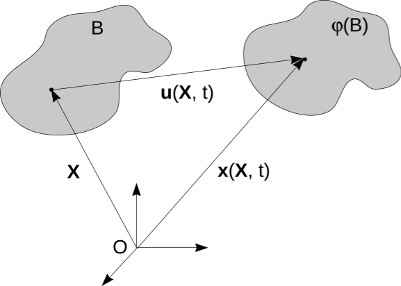
Let us consider a body in its initial configuration B. Each point of it can be described by its coordinates X = (X1, X2, X3). In its deformed configuration j(B), these points are defined by their coordinates x(X) = (x1, x2, x3). The displacement vector u(X) of the point X due to deformation is obviously defined as

u(X) = x(X) - X.

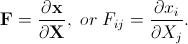
Let us also introduce the deformation gradient tensor as follows:

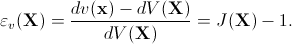
It can be shown that its determinant J(X) = det(F) describes the volume of a small region around the point x in the deformed configuration divided by its volume in the initial configuration: dv(x) = J * dV(X). Thus the volumetric strain in the point X can be defined as follows:

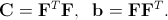
Given the deformation gradient tensor F, the left Cauchy-Green deformation tensor C and the right Cauchy-Green deformation tensor b can be introduced as follows:

Strain and stress tensors

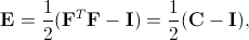
Using the deformation gradient tensor as well as the right and left Cauchy-Green deformation tensors defined in the previous section, the following strain tensors can be introduced. The Green-Lagrangian strain tensor is defined in the initial configuration:

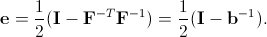
where I is the unit matrix. In contrast, the Almansi strain tensor is defined in the deformed configuration:

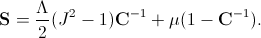
The mechanical solver employs the Neo-Hookean material model. This model defines the following relation between the 2nd Piola-Kirchhoff stress tensor and the deformation of the model:

The 2nd Piola-Kirchhoff stress tensor is defined in the initial configuration. Its counterpart in the deformed configuration is the Cauchy stress tensor:

These relations contain material parameters which can be directly computed from the Young's modulus and Poisson's ratio employed by the linear solver:

Exactly like in the linear case, the stationary mechanical computation implies the solution of the impulse conservation equation:

where Div is the divergence operator in the initial configuration and f the external force.


Copyright © 2006 - 2013 微波EDA网, All Rights Reserved 业务联系：mweda@163.com