|
|
|
| 首页 >> CST教程 >> CST2013在线帮助系统 |
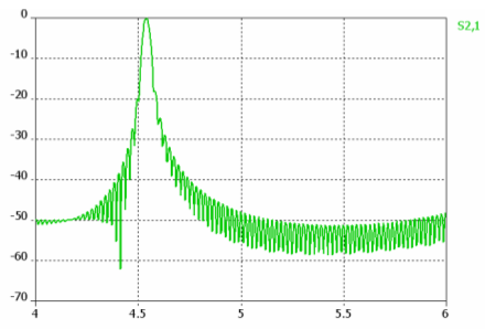
AR-Filter OverviewThe performance of the high frequency transient solver can be significantly reduced when strongly resonating devices are simulated. The main reason for this is that calculating the S-parameters using a Fourier Transform requires the time signals to have sufficiently decayed to zero; otherwise a truncation error will occur. The Auto-regressive filter (AR-filter) is a signal processing method to predict time signals to save simulation time.Especially for highly resonant devices, a ringing in the time signals may occur so that the signals decay very slowly and therefore require long simulation times for accurate Fourier Transforms.The Auto-regressive filter (AR-filter) must be adjusted properly to obtain accurate results. It is possible to apply the AR-filter to the time signals of ports, probes, current and voltage monitors. The following description and hints will help you simulate high resonant structures by using the time domain solver.OverviewDetermine AR-Filter SettingsIf an S-parameter calculation is performed using time signals which still exhibit some oscillation, a ripple will appear on the S-parameters as shown in the picture below:
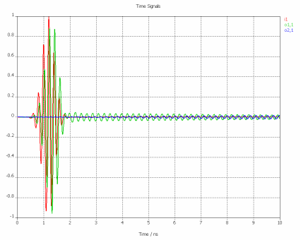
Please note that the curve’s minimum or maximum locations (i.e. the position of the resonance frequencies) are not affected by the ripple, so if this is the only information needed from the simulation, the truncation error may be tolerated. Otherwise, the usage of the AR-filter feature may be useful. The idea of this technique is to train an auto-regressive (AR) filter by using a short interval of the time signals. Afterwards, the AR-filter is used to predict the signal for the next time steps. Once the prediction and the actual simulation agree sufficiently, the AR-filter contains all relevant information about the device. Therefore the simulation can be stopped, and the S-parameters can be derived mathematically from the AR-filter’s representation. The AR-filter is only capable of approximating exponentially damped signals. Therefore the starting point for the AR-filter calculation always should be at the first maximum after the stimulation has finished. The following two pictures shows typical time signals of resonating structures. The first one is decaying rather quick, the first time step should be defined as indicated beyond the first maximum:
The next picture shows a typical time signal for a strongly resonating structure. Here the time signal is decaying very slowly, the first time step could be defined around 2 ns:
Once such a simulation is completed (or aborted
manually), you can enter the AR-filter dialog box by choosing Post Processing:
Signal Post Processing
First, you should always press the Defaults button to let the dialog optimize its settings for currently available time domain data. Next, you should carefully inspect the signals as described and determine the time when the excitation pulse has vanished. In the second example above, this may be at around 2 ns. Afterwards, enter this time in the First time step field to start the AR-filter analysis when the device’s response is dominated by the resonant parts only. Now check the order of the AR-filter. The maximum filter order that should be used depends on the complexity of the analyzed time signal. For structures that are dominated by only one or two modes, it may be sufficient to use filters of order 5, while others may require 60 or even 80 filter coefficients. As an example the following picture was calculated properly with a 5-order filter:
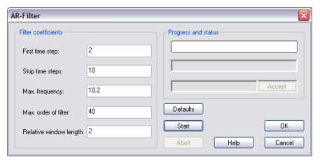
If the signal contains a few resonances only (e.g. you are expecting only a few poles inside the frequency band of interest), you should start with a Max. order of filter set to 40. Increasing the window length might improve accuracy without using a higher filter order, but it also takes more time to calculate a filter. You should increase the relative window length in the range of 2.0 to 4.0 if no filter of desired order can be found. Here, we keep the default value of 2 and after making all discussed settings, the dialog box should look as follows:
Now click the Start button to perform the AR-filter analysis. Once the computation is finished, a dialog box will appear containing handy information. Analyzing AR-Filter ResultsA header provides information about the AR-filter’s settings and the currently investigated time signal:
=================================================================== Analysis 1 of 2 for stimulation port 1, mode 1 =================================================================== First time step : 2.001828e+000 ns Skip time steps : 10 Max. frequency : 1.020000e+001 GHz Max. order of filter : 40 Relative Window length: 2.000000e+000 Input signal samples : 7913 Input signal length : 5.617186e+001 ns
The AR-filter information is extracted from a window that moves along the time signal. The following information displays the bounds of this window for each evaluation step and the energy error of the resulting filter approximation. This error should ideally be below 1e-3 in order to obtain good accuracy. Moreover, it is important to check if a stable filter of maximum order was found (if not, you may increase the relative window length).
------------------------------------------------------------------------------- step | window range | rel. wnd. | filter | energy | pulses to | ns | length | order | error | calculate ------|---------------------------|-----------|--------|-----------|----------- 1 | 1.7747e+000 - 4.6141e+000 | 2.50 | 32 | 4.83e-007 | 1.95e+000 2 | 1.8457e+000 - 4.6851e+000 | 2.50 | 33 | 4.80e-007 | 1.98e+000 3 | 1.9166e+000 - 4.7561e+000 | 2.50 | 30 | 1.00e-006 | 2.01e+000 4 | 1.9876e+000 - 4.8271e+000 | 2.50 | 30 | 1.14e-006 | 2.04e+000 5 | 1.4907e+000 - 4.8981e+000 | 3.00 | 36 | 8.60e-007 | 2.07e+000 6 | 1.5617e+000 - 4.9691e+000 | 3.00 | 37 | 1.38e-006 | 2.10e+000 7 | 1.6327e+000 - 5.0401e+000 | 3.00 | 35 | 2.68e-006 | 2.13e+000 ------------------------------------------------------------------------------- filter step 2 used for further calculations ------------------------------------------------------------------------------- =================================================================== Analysis 2 of 2 for stimulation port 1, mode 1 =================================================================== First time step : 2.001828e+000 ns Skip time steps : 10 Max. frequency : 1.020000e+001 GHz Max. order of filter : 40 Relative Window length: 2.000000e+000 Input signal samples : 7913 Input signal length : 5.617186e+001 ns ------------------------------------------------------------------------------- step | window range | rel. wnd. | filter | energy | pulses to | ns | length | order | error | calculate ------|---------------------------|-----------|--------|-----------|----------- 1 | 6.3888e-001 - 4.6141e+000 | 3.50 | 1 | 1.00e+000 | 1.95e+000 2 | 2.4136e+000 - 4.6851e+000 | 2.00 | 31 | 6.54e-009 | 1.98e+000 3 | 2.4845e+000 - 4.7561e+000 | 2.00 | 33 | 1.49e-009 | 2.01e+000 4 | 2.5555e+000 - 4.8271e+000 | 2.00 | 32 | 7.95e-010 | 2.04e+000 5 | 2.6265e+000 - 4.8981e+000 | 2.00 | 32 | 1.91e-010 | 2.07e+000 6 | 2.6975e+000 - 4.9691e+000 | 2.00 | 31 | 1.23e-009 | 2.10e+000 7 | 2.7685e+000 - 5.0401e+000 | 2.00 | 31 | 4.99e-010 | 2.13e+000 8 | 2.8395e+000 - 5.1111e+000 | 2.00 | 31 | 1.53e-010 | 2.16e+000 9 | 2.9105e+000 - 5.1820e+000 | 2.00 | 30 | 4.50e-010 | 2.19e+000 10 | 2.4136e+000 - 5.2530e+000 | 2.50 | 37 | 3.76e-010 | 2.22e+000 11 | 2.4845e+000 - 5.3240e+000 | 2.50 | 37 | 4.13e-010 | 2.25e+000 12 | 2.5555e+000 - 5.3950e+000 | 2.50 | 35 | 1.61e-009 | 2.28e+000 13 | 2.6265e+000 - 5.4660e+000 | 2.50 | 37 | 4.10e-010 | 2.31e+000 ------------------------------------------------------------------------------- filter step 8 used for further calculations -------------------------------------------------------------------------------
In this example, excellent filter accuracy can be obtained for both time signals. As a next step, the S-parameters are calculated from the AR-filter’s representation, and the energy balance of the S-matrix is evaluated. The following lines show information about how well the energy conservation is maintained.
=========================================================== Stimulation at port 1 (mode 1) Average deviation in s-parameter energy balance: 6.094664e-004 Maximum deviation in s-parameter energy balance: 2.756003e-001 =========================================================== =================================================================== Maximum deviation in s-parameter energy balance = 0.2756 (regarding all successfull filter runs) ===================================================================
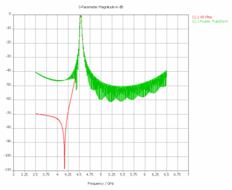
It can be seen from these data that the average energy error is sufficiently small, but the maximum error is much larger. This happens quite often if the S-parameters show some very sharp resonances and the locations of the poles and zeros in the various S-parameter curves do not match exactly. In most cases, this inaccuracy can simply be ignored. The AR-filter’s results are added to the navigation tree in the same way as the standard S-parameter curves, but marked by an extension ”(AR)”. The following picture shows an original S-parameter with its AR-filter approximation (the curves may easily be overlaid using the Copy / Paste feature of curves in the navigation tree):
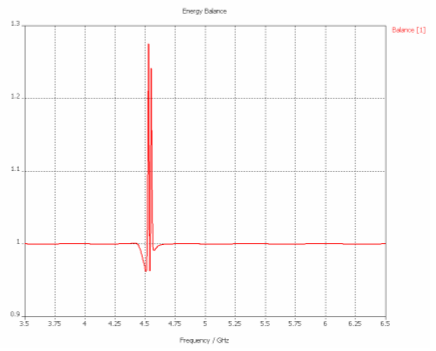
Furthermore, the balance of the AR-filter S-parameters looks as follows:
The energy balance is very close to one for the most part of the spectrum. Even if the balance is significantly disturbed close to the location of the peaks, this inaccuracy can hardly be seen in the S-parameter results. In case of loss-free (no conductivity / open boundaries) structures, the energy balance should be one over the complete frequency range. If there is a strong variation on the energy balance over a wide frequency interval you should run a new AR-filter calculation with more filter coefficients and/or another first time step. The energy balance indicates whether the accuracy of an S-parameter calculation is sufficient. As an example the following picture demonstrates a bad energy balance: Taking a closer look at the AR-filter output shown above, you can check that the AR-filter calculation uses time windows up to a maximum time of 5.466ns. This means that at least this maximum time needs to be simulated. In order to minimize the simulation time, you may consider decreasing the filter’s order. This in turn would require shorter time windows. Every system, however, needs a certain minimum number of poles to be described properly. If the order is set lower than the actual order of the device’s response, accuracy will be degraded significantly. Performing an AR-filter calculation using a filter order of only 10 for this example would yield the following output:
===========================================================----- Stimulation at port 1 (mode 1) Average deviation in s-parameter energy balance: 3.669134e-003 Maximum deviation in s-parameter energy balance: 1.463659e+000 ===========================================================----- =================================================================== Maximum deviation in s-parameter energy balance = 1.46366 (regarding all successful filter runs) ===================================================================
Large deviations of the energy balance (e.g. significantly larger than 0.5) usually indicate highly inaccurate results. Another criterion for the quality of the AR-filter approximation is the energy error shown in the dialog box after the AR-filter computation has finished:
The energy error shown here should usually be lower than 1e-3 for reliable results (it was 1.5e-10 for a filter order of 40).
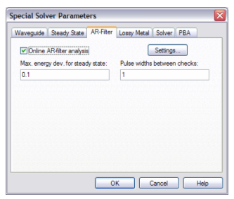
If the AR-filter yields inaccurate results and you cannot improve its quality by increasing the Max. order of filter and the First time step settings, you should try to follow these guidelines: 1. Avoid including DC (frequency = 0) in the simulation. The AR-filter approximation is most critical for very low frequencies. 2. Use sufficiently small simulation bandwidths. Especially for narrow band filters, very small ranges of the spectrum contain most of the significant device information. 3. It rarely makes sense to use filter orders of more than 100-150. It may be better to increase the First time step setting instead or to reduce the simulation frequency range. Online AR-FilterIt is possible to apply the AR-filter online to the S-Parameters. During the transient simulation, the AR-filter calculation will frequently be performed (Pulse widths between checks), and the balance of the resulting S-parameters will be checked. If the balance error turns out to be better than Max. energy dev. for steady state, the transient simulation will automatically stop. Simulation time can be reduced significantly by this procedure. In addition, if the AR-filter has been successfully applied to a device in post processing, then it can be used with the settings of the successful run as an Online AR-filter for subsequent calculations such as parameter sweeps or optimizations. This feature can be activated from the Specials dialog box (AR-Filter tab) from within the transient solver dialog box:
You can check the Online AR-filter analysis box and specify its parameters by clicking the Settings... button. If an AR-filter calculation has been previously performed in post-processing, its parameters will be retained here. Please note, that the Online AR-filter analysis is only applied to the signals corresponding to S-Parameters. The spectra of the signals from monitors and probes are not accessed online but can be predicted as a post processing step after a successful calculation.
AR-Filter, Solver Specials AR-Filter
HFSS视频教程 ADS视频教程 CST视频教程 Ansoft Designer 中文教程 |
|
Copyright © 2006 - 2013 微波EDA网, All Rights Reserved 业务联系:mweda@163.com |
|