![]()
![]()
|
Tetrahedral mesh: |
|
|
Eigenmode Solver: |
|
|
Hexahedral mesh (AKS): |
|
|
Eigenmode Solver: |
|
|
Hexahedral mesh (JDM): |
|
|
Eigenmode Solver: |
|
Geometric Construction and Solver Settings
Introduction and Models Dimensions
Eigenmode Calculation with Tetrahedral mesh
Eigenmode Visualization and Q-Factor Calculation
Eigenmode Calculation with AKS
Eigenmode Calculation with JDM
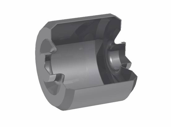
This tutorial demonstrates how to simulate resonator devices. As a typical example, you will learn how to calculate the eigenmodes of an air filled cavity. The following explanations can be applied to other resonators as well.
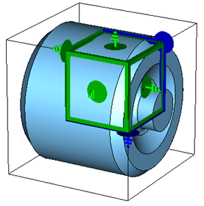
Due to its rotational symmetry, the cavity can be easily modeled by rotating a cross section profile around an axis. Furthermore, due to a second symmetry, it is sufficient to draw half of the profile and mirror the structure afterwards to build the full model. After the model is constructed, the analysis process is quite simple. This tutorial will show you how to calculate and visualize a number of eigenmodes for this resonator. In addition, the Q-factors will be calculated.
Please note: The CST MICROWAVE STUDIO Eigenmode solver license is required for this tutorial. If it is not available, please contact your distribution partner.
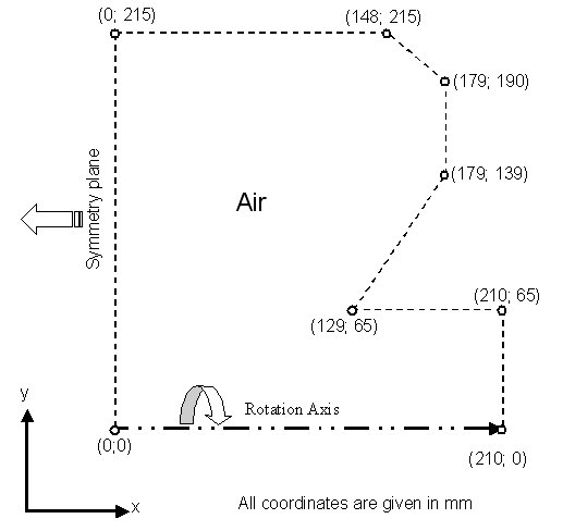
The cross section polygon is shown below. Please note than only half of the profile needs to be drawn because of the depicted symmetry. The coordinates are given in mm for each of the polygons points.
The following sections will guide you through the construction of the cavity's model. Please make sure that you carefully complete each step before you proceed to the next one.
o Create a New Project
After launching the CST STUDIO SUITE
you will enter the start screen showing you a list of recently opened
projects and allowing you to specify the application which suits your
requirements best. The easiest way to get started is to configure a project
template which defines the basic settings that are meaningful for your
typical application. Therefore click on the Create
Project button ![]() in the New Project section.
in the New Project section.
Next you should choose the application area, which is Microwaves & RF for the example in this tutorial and then select the workflow by double-clicking on the corresponding entry.

For the filter structure, please select
Circuits & Components ![]() Waveguide & Cavity Filters
Waveguide & Cavity Filters ![]() Eigenmode
Eigenmode ![]() .
.
This template by default sets the units to mm and GHz, the background material to perfect electrically conduction (PEC, which is the default) and all boundaries to be perfect electrical conductors.
After clicking the Next button, you can give the project template a name and review a summary of your initial settings:
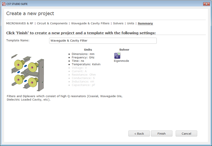
Finally click the Finish button to save the project template and to create a new project with appropriate settings. CST MICROWAVE STUDIO will be launched automatically due to the choice of the application area Microwaves & RF.
Please note: When you click again on the File: New and Recent you will see that the recently defined template appears below the Project Templates section. For further projects in the same application area you can simply click on this template entry to launch CST MICROWAVE STUDIO with useful basic settings. It is not necessary to define a new template each time. You are now able to start the software with reasonable initial settings quickly with just one click on the corresponding template.
Please
note: All settings made for a project template can be modified
later on during the construction of your model. For example, the units
can be modified in the units dialog box (Home:Settings ![]() Units
Units ![]() ) and the solver type can be selected
in the Home:Simulation
) and the solver type can be selected
in the Home:Simulation ![]() Start Simulation drop-down
list.
Start Simulation drop-down
list.
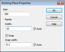
o Set Working Plane Properties
Before you start entering the cavity's
shape, you should set the working plane to be large enough to contain
the models dimensions. The dialog box can be accessed by selecting
View:Visibility
![]() Working Plane
Working Plane ![]()
![]() Working Plane Properties.
Working Plane Properties.
The largest coordinate value is 215 mm, so a working plane size of 250 mm will suffice. Enter this value in the Size field and set the Raster Width to 10 mm in order to obtain a reasonably fine grid on the drawing plane. Please note that all geometric settings are in mm because the current geometry unit is set to mm (displayed in the status bar.)
o Create Figure of Rotation
After these preparatory steps have been
completed, you can now start drawing the figure of rotation. Because
the cross section profile is a simple polygon, you do not need to use
the curve modeling tools here (please refer to the Workflow and Solver Overview
manual for more information on this advanced functionality). For
polygonal cross sections, it is more convenient to use the figure of rotation
tool, activated by selecting
Modeling: Shapes ![]() Extrusions
Extrusions
![]()
![]() Rotate
Rotate ![]() .
.
Since no face has been previously picked, the tool will automatically enter a polygon definition mode and request that you enter the polygons points. You can do this either by double-clicking on each points coordinates on the drawing plane, or by entering the values numerically. Because the latter approach may be more convenient, we suggest pressing the Tab key and entering the coordinates in the dialog box. All polygon points can thus be entered according to the following table (whenever you make a mistake, you can delete the most recently entered point by pressing the Backspace key):
|
Point |
X |
Y |
|
1 |
0 |
0 |
|
2 |
210 |
0 |
|
3 |
210 |
65 |
|
4 |
129 |
65 |
|
5 |
179 |
139 |
|
6 |
179 |
190 |
|
7 |
148 |
215 |
|
8 |
0 |
215 |
|
9 |
0 |
0 |
After the last point has been entered, the polygon will then be closed. The Rotate Profile dialog box will then automatically appear.
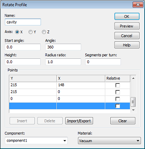
This dialog box allows you to review the coordinate settings in the table. If you encounter any mistakes you can easily change the values by double-clicking on the incorrect coordinates entry field.
The next step is to assign a specific Component and a Material to the shape. In this case, the default settings with component1 and Vacuum are practically appropriate.
Please note: The use of different components allows you to combine several solids into specific groups, independent of their material behavior. However, here it is convenient to construct the complete cavity as a representation of one component.
Finally, you should assign a proper Name (e.g. cavity) to the shape and press the OK button in order to create the solid.
o Smart Pick ![]() and Blend Edge
and Blend Edge ![]()
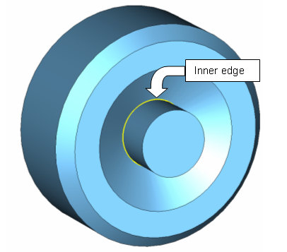
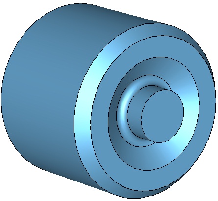
Sharp edges inside cavities are best avoided because strong field singularities will occur at these edges. Therefore, the sharp inner edge (shown on the picture below) should be blended.
The first step towards blending the
edge is to pick the edge in the model by entering the smart pick mode
via
Modeling: Picks ![]() Picks
Picks ![]() (shortcut S)
in the main view
window. Once this mode is active, which is indicated by edges and
points in the model being highlighted, you can easily double-click at
the inner edge. If the edge is hidden, you can rotate the view using
the view changing tools as explained in the Workflow
and Solver Overview manual. Sometimes it
is also advantageous to switch the drawing mode to wireframe by selecting
View: Visibility
(shortcut S)
in the main view
window. Once this mode is active, which is indicated by edges and
points in the model being highlighted, you can easily double-click at
the inner edge. If the edge is hidden, you can rotate the view using
the view changing tools as explained in the Workflow
and Solver Overview manual. Sometimes it
is also advantageous to switch the drawing mode to wireframe by selecting
View: Visibility ![]() Wire Frame
Wire Frame ![]() , or use the corresponding shortcut Ctrl+w.
, or use the corresponding shortcut Ctrl+w.
Once the proper edge has been selected, the model should look as follows:
If you accidentally picked the wrong
edge, you can delete all picks using
Modeling: Picks ![]() Clear Picks
Clear Picks ![]() (shortcut d)
and try again.
(shortcut d)
and try again.
The next step is to blend the selected
edge. Therefore, press
Modeling: Tools ![]() Blend
Blend ![]() .
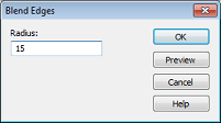
Afterwards, a dialog
box will open where you can set the Radius of the blend to 15 mm.
.
Afterwards, a dialog
box will open where you can set the Radius of the blend to 15 mm.
Finally press the OK button to apply the blend. The structure should then look as follows:
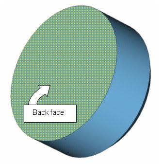
o Mirror the Structure to Model the Entire Cavity
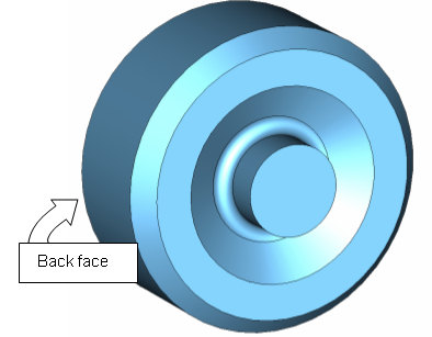
Thus far you have successfully modeled half of the cavity. The easiest way to obtain the full model is to mirror this structure at the planar back face.
The first step is to define the mirror
plane by picking the corresponding face in the model. Therefore,
enter the smart pick mode via
Modeling: Picks ![]() Picks
Picks ![]() .
.
Once the smart pick mode is active, you should double-click on the planar back face as shown in the picture above. If the face is hidden by the structure, you can use the view changing tools as explained in the Workflow and Solver Overview manual. After the face has been selected, the model should look as follows:
You should now select the cavity solid by double-clicking it. Please confirm that its name becomes highlighted in the navigation tree.
The next step is to use the transform
tool to create the mirrored shape by pressing
Modeling:
Tools ![]() Transform
Transform ![]() Mirror
Mirror
![]() .
.
In the dialog box that appears the Operation Mirror is selected. The mirror planes' coordinates will then be automatically set according to the previously-picked back face of the cavity, so you do not need to change any of the coordinate settings.
![]()
Because the transformation will create a new shape by mirroring the existing one, you have to select the Copy option. Furthermore, the original shape should also be combined with the mirrored one to form a single shape. Thus, the Unite option must also be switched on.
Finally, you should press the OK button to create the entire cavity shown below:
After you have successfully modeled the cavity's geometry, you need to specify some solver settings, such as frequency range and boundary conditions, before you can finally start the solver to calculate the eigenmodes.
o
Define the Frequency Range ![]()
For this device, the first five resonance
frequencies are estimated to be below 1.5 GHz. Open the frequency
range dialog box either by pressing
Simulation:
Settings
![]() Frequency
Frequency
![]() .
In this dialog box you should set the upper frequency limit to 1.5 (please
recall that the frequency unit has been set to GHz as shown in the status
bar).
.
In this dialog box you should set the upper frequency limit to 1.5 (please
recall that the frequency unit has been set to GHz as shown in the status
bar).
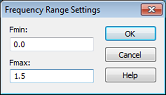
Finally, press the OK button to store these settings.
o Define Boundary Conditions and Symmetries
You should always check the boundary
and symmetry conditions before starting the solver. This is most
easily accomplished by entering the boundary definition mode by pressing
Simulation:
Settings ![]() Boundaries
Boundaries ![]() The boundary conditions will
then become visualized in the main view. Due to the previously selected
template, all boundary conditions are set to electric, meaning that the
structure is embedded in a perfect electrically conducting housing.
These defaults (which have been set by the template) are appropriate for
this example.
The boundary conditions will
then become visualized in the main view. Due to the previously selected
template, all boundary conditions are set to electric, meaning that the
structure is embedded in a perfect electrically conducting housing.
These defaults (which have been set by the template) are appropriate for
this example.
Assume that you are only interested in those modes that have longitudinal electric field components along the x-axis of the device. This a priori knowledge about the fields can be used to speed up the calculation significantly by informing the solver about these symmetry conditions.
Please enter the symmetry plane definition mode by activating the Symmetry Planes tab in the dialog box.
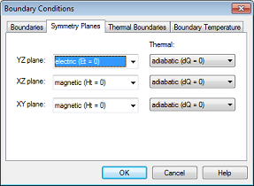
By setting the symmetry planes XY and XZ to magnetic, you force the solver to only calculate fields that have no magnetic field tangential to these planes (thereby forcing the electric field to be tangential to these planes). Additionally, you can set the YZ symmetry plane to electric, which implies that the electric field is forced to be normal to this plane.
After these settings have been made, the structure should look as follows:
Finally press the OK button to complete this step.
In general, you should always make use of symmetry conditions whenever possible in order to reduce calculation times.
After completing all of the above steps, you are ready to start the eigenmode calculation.
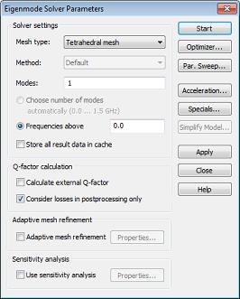
The Eigenmode solver in CST MICROWAVE STUDIOТЎ offers the possibility to choose between tetrahedral and hexahedral meshes, with the former being the default.
Please enter the eigenmode
solver control dialog box more by pressing
Home:
Simulation ![]() Start Simulation
Start Simulation
![]() .
The tetrahedral mesh is already selected in the Solver settings frame.
.
The tetrahedral mesh is already selected in the Solver settings frame.
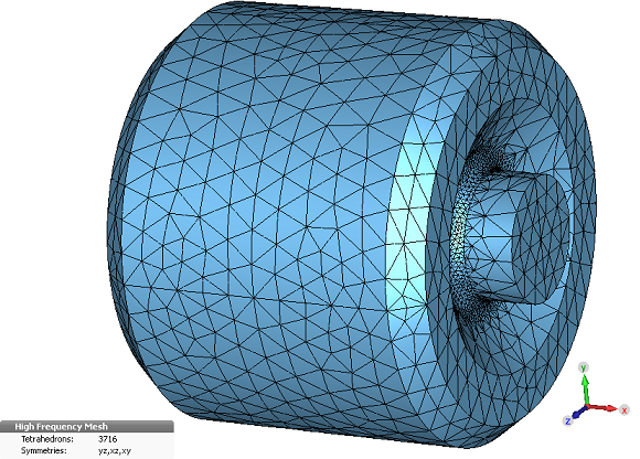
Finally, press the Start button, and the solver will generate the tetrahedral mesh as a first step. Click on Mesh Control in the navigation tree to view the curved tetrahedral mesh.
o Eigenmode Visualization
The eigenmode results can be accessed
by selecting the corresponding item in the navigation tree from the 2D/3D
Results ![]() Modes
folder. The field patterns for each mode will be stored in subfolders
named Mode N where N represents the mode number.
Modes
folder. The field patterns for each mode will be stored in subfolders
named Mode N where N represents the mode number.
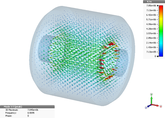
To visualize the electric field of the
first mode, select the corresponding item from the navigation bar: 2D/3D
Results ![]() Modes
Modes ![]() Mode 1
Mode 1![]() e.
The result data will then be visualized in a three dimensional vector
plot as shown in the above picture.
e.
The result data will then be visualized in a three dimensional vector
plot as shown in the above picture.
Please note: The field amplitudes of the modes will always be normalized such that each mode contains a total energy of 1 Joule.
In many cases, it is more important
to visualize the fields in a cross section plane. Therefore, please switch
to the 2D field visualization mode by pressing
2D/3D Plot:
Sectional View ![]() 3D Fields on 2D Plane
3D Fields on 2D Plane ![]() .
The field data should
then be visualized and appear similar to the picture below. Please
refer to the Workflow
and Solver Overview manual or press the F1
key for online help to obtain more information on field visualization
options.
.
The field data should
then be visualized and appear similar to the picture below. Please
refer to the Workflow
and Solver Overview manual or press the F1
key for online help to obtain more information on field visualization
options.
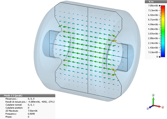
In addition to the graphical field visualization, some information text containing maximum field strength values and resonance frequencies will also be shown in the main window.
o Q Factor Calculation
The eigenmodes internal Q-factors, which
are an important quantity for cavity design, can be easily derived from
the field patterns. Open the loss and Q-factor calculation dialog
box by selecting
Post Processing: 2D/3D Field Post Processing ![]() Loss and Q
Loss and Q
![]() .
.
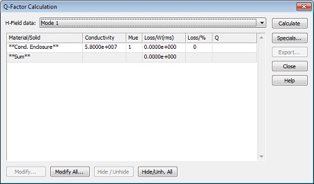
The only setting that requires specification here is the conductivity of the enclosing metal. By default, the conductivity of the Cond. Enclosure is set to copper (5.8e7 S/m).
You may change this setting by clicking on the first row and selecting the Modify button that opens the following dialog box:
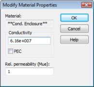
In this example, you can set the Conductivity value to silver (6.16e7 S/m) and press the OK button.
Back in the loss and Q factor calculation dialog box you should now select the desired Mode from the H-Field data list, e.g. the fundamental mode Mode 1. Finally, press the Calculate button to obtain the Q factor value.
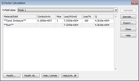
The Q-factor is calculated to be 4.36"104 for the fundamental mode.
o Calculating the Eigenmodes Using Fully Automatic Solver Settings
Please enter the eigenmode
solver control dialog box more by pressing
Home:
Simulation ![]() Start Simulation
Start Simulation
![]() .
Please change the mesh type to hexahedral in the Solver settings frame.
.
Please change the mesh type to hexahedral in the Solver settings frame.
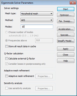
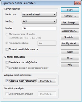
The only setting that commonly needs to be specified here is the number of Modes to be calculated. The solver will then calculate this number of modes starting from the lowest resonance frequency. It is usually advantageous to specify more modes than you are actually searching for. Thus, assuming that you want to calculate the first five modes in this example, you should advise the eigenmode solver to calculate 10 modes. Afterwards, press the Start button to run the simulation.
Due to the Perfect Boundary ApproximationТЎ, the number of mesh cells required for discretizing this example is quite small (roughly 7700). This, in fact, corresponds to a system of equations consisting of about 23,100 unknowns. Calculating eigenmodes for such a system takes only a few minutes to complete on a modern PC.
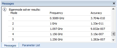
After the solver has finished its work, the resonance frequencies of the first ten modes are displayed in the result window:
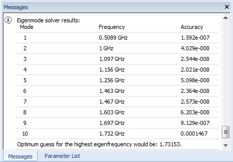
The accuracy for the mode solution is excellent for all the required modes. A mode with an accuracy of less than 1e-3 can usually be considered sufficiently accurate.
In order to review the solver time required
to achieve these results, you can display the solver log-file by selecting
Simulation:
Solver
![]() Logfile
Logfile ![]() . Please scroll
down the text to obtain the following timing information (the actual values
may vary depending on the speed of your computer):
. Please scroll
down the text to obtain the following timing information (the actual values
may vary depending on the speed of your computer):
Mesh generation time : 3 s
Solver time : 8 s
Total time : 11 s
--------------------------------------------------------------
o Optimizing the Performance for Subsequent Calculations
To this point, you have successfully calculated the eigenmodes for this device in a reasonable amount of time. However, if you intend to make parametric studies it may be advantageous to speed up the solver for subsequent runs.
This performance tuning step is quite simple: The eigenmode solver can make use of a guess for the highest eigenmode frequency you are looking for. The eigenmode solver automatically determines this guess from a previous calculation and prints the result in the log-file. This information is shown right below the timing information:
--------------------------------------------------------------
Optimum guess for the highest eigenfrequency would be: 1.73153
--------------------------------------------------------------
In order to demonstrate how this information
can be used for improving the solvers speed, you should now recalculate
the eigenmodes to compare the time required for the simulation.
Please enter the eigenmode solver control dialog box once more by pressing
Home:
Simulation ![]() Start Simulation
Start Simulation
![]() .
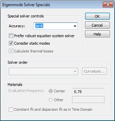
In this dialog box, press the Specials
button in order to open a dialog box for more advanced settings:
.
In this dialog box, press the Specials
button in order to open a dialog box for more advanced settings:
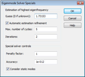
Once you have obtained a guess for the highest eigenfrequency of interest (here 1.73153 GHz), you can enter this value in the Guess field. If you dont know this value, just enter zero to let the solver estimate this value automatically. After pressing the OK button in this dialog box you can restart the eigenmode solver by pressing the Start button.
Again, a progress bar will appear informing you of the status of your calculation. Please note that there is no need for recalculating the matrix because the structure has not been changed.
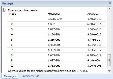
The solver will finish its work after a short time, giving the same results as before for the eigenfrequencies. The timing information in the log-file should look similar to the data below:
Mesh generation time : 0 s
Solver time : 5 s
Total time : 5 s
--------------------------------------------------------------
If you now compare the solver times, you can see that specifying the guess for the highest eigenfrequency could speed up the solution process.
Please remember that these steps are only made in order to illustrate how to speed up the solver for parametric sweeps or optimizations. The accuracy of the solution will also be excellent using the fully automatic procedure without this additional setting. For a single analysis of a particular device, this performance tuning is not necessary, but it might further improve the accuracy:
The eigenmode calculation is mainly affected by two sources of numerical inaccuracies:
1. Numerical errors introduced by the iterative eigenmode solver.
2. Inaccuracies arising from the finite mesh resolution.
In the following sections we provide hints on how to minimize these errors and achieve highly accurate results.
o Accuracy of the Numerical Eigenmode Solver
The first type of error is always quantified as Accuracy for each mode after the calculation has finished. The modes can usually be considered sufficiently accurate for most practical applications if the mode accuracy is below 1e-3.
The results can be improved by specifying a proper guess for the highest eigenmode frequency of interest and by increasing the number of iterations for the eigenmode solver. Specifying more than five iterations does not typically improve the results. Sometimes higher order modes are calculated with a lower accuracy than lower order modes. In many cases it may be advantageous to calculate more modes than you are actually looking for, in order to improve the accuracy of the desired (lower) ones.
Please note: Here, we calculate the modes with the AKS eigenmode solver. In the next section the JDM solver is used. In contrast to the AKS eigenmode solver, the JDM solver requires no guess of the highest eigenfrequency and the eigenmodes are calculated to a prescribed accuracy.
o Effect of the Mesh Resolution on the Eigenmode Accuracy
The inaccuracies arising from the finite mesh resolution are usually more difficult to estimate. The only way to ensure the accuracy of the solution is to increase the mesh resolution and recalculate the eigenmodes. If the desired results (e.g. eigenmode frequencies, Q-factors) do not significantly change after increasing the mesh density, then convergence has been achieved.
In the above example, you have used
the default hexahedral mesh that has been automatically generated by an expert system.
The easiest method of testing the accuracy of the results is to use the
fully automatic mesh adaptation that can be switched on by checking the
Adaptive mesh refinement option in the solver control dialog box
(Home:
Simulation ![]() Start Simulation
Start Simulation
![]() ):
):
After activating the adaptive mesh refinement tool, the Properties button becomes active. Press this button to open the mesh refinement properties dialog box:
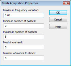
Because you are only interested in the first five modes of this structure, you should change the Number of modes to check to 5 in order to focus the mesh refinement procedure on these modes. Afterwards, you can close this dialog box by pressing the OK button.
Back in the solver dialog box, you can now start the eigenmode solver again by pressing the Start button. After a couple of minutes, during which the solver is running through mesh adaptation passes, the following dialog box will appear:
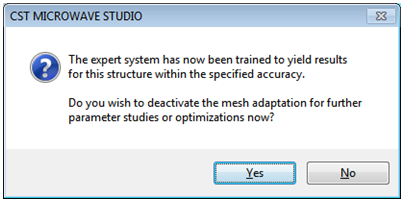
This dialog box notifies you that the desired accuracy limit (1% by default) could be met by the adaptive mesh refinement. Since the expert systems settings have been adjusted to achieve 1% accuracy, you may switch off the adaptation procedure for subsequent calculations (e.g. parameter sweeps or optimizations).
You should now confirm the deactivation of the mesh adaptation by pressing the Yes button. The converged results for the eigenmode frequencies will then be shown in the result window.
After the mesh adaptation procedure
is complete, you can visualize the maximum relative difference in the
eigenmode frequencies for two subsequent passes by selecting 1D Results
![]() Adaptive Meshing
Adaptive Meshing
![]() Error
from the navigation tree:
Error
from the navigation tree:
As evident from the above plot, the maximum devation of the eigenmodes frequencies is below 0.14%, indicating that the expert system based meshing would have been fine for this example, even without running the mesh adaptation procedure.
The eigenmode solver accuracies achieved
for the modes during the mesh adaptation can be visualized by selecting
1D Results ![]() Adaptive Meshing
Adaptive Meshing ![]() Mode Accuracies from the navigation tree:
Mode Accuracies from the navigation tree:
The above plot shows that all mode accuracies
for both passes are fine. Finally, you can visualize the convergence
process of the mode frequencies by clicking on 1D Results ![]() Adaptive Meshing
Adaptive Meshing
![]() Mode Frequencies:
Mode Frequencies:
Inspection of the above plot confirms that the results are quite stable.
The major advantage of the expert system based mesh refinement procedure over traditional adaptive schemes is that the mesh adaptation needs to be carried out only once for each device in order to determine the optimum settings for the expert system. There is then no need for time consuming mesh adaptation cycles during parameter sweeps or optimization.
CST MICROWAVE STUDIOТЎ offers
the possibility to choose the JDM eigenmode solver. This solver
is recommended only if a small number of eigenmodes are required (5 modes
or less). Since this is a tutorial, it is convenient to reset the
mesh settings to the initial values of the mesh adaptation to speed up
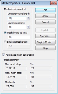
the calculation. Open the Mesh Properties dialog for the hexahedral
mesh by selecting
Home:
Mesh![]() Global Properties
Global Properties
![]() :
and set both Lines per wavelength
and Lower mesh limit equal to 10.
:
and set both Lines per wavelength
and Lower mesh limit equal to 10.
There may be old results present from the previous solver run that will be overwritten when changing the mesh. In this case, the following warning message appears:
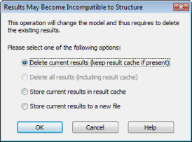
Press OK to acknowledge deletion of the previous results.
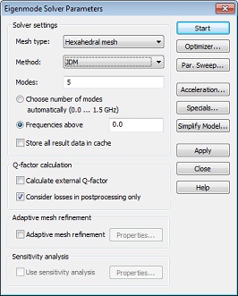
The solvers parameters are specified
in the solver control dialog box that can be opened again by selecting
Home:
Simulation ![]() Start Simulation
Start Simulation
![]() .
Select from the Method drop down menu the eigenmode
solver JDM and reduce the number of Modes to 5. With these
settings the solver will calculate 5 modes starting from the lowest resonance
frequency.
.
Select from the Method drop down menu the eigenmode
solver JDM and reduce the number of Modes to 5. With these
settings the solver will calculate 5 modes starting from the lowest resonance
frequency.
Before starting the eigenmode solver, you may select the Specials button in order to change the desired accuracy for the eigenmodes. In this case, the value of 1e-6 is sufficient and you can leave the box unchanged by pressing the OK button.
Finally, press the Start button. A few progress bars will appear in the status bar again, keeping you informed of the current status of your calculation (e.g. matrix calculation, eigenmode analysis). After the solver has finished, the resonance frequencies of the first five modes are displayed in the main view.
In order to review the solver time required
to achieve these results, you can display the solver log-file by selecting
Results ![]() View Logfiles
View Logfiles ![]() Solver Logfile from the main menu. Please scroll
down the text to obtain the following timing information (the actual values
may vary depending on the speed of your computer):
Solver Logfile from the main menu. Please scroll
down the text to obtain the following timing information (the actual values
may vary depending on the speed of your computer):
Mesh generation time : 3 s
Solver time : 10 s
Total time : 13 s
--------------------------------------------------------------
The solver time required for the calculation is comparable to the AKS eigenmode solver.
Please note: In contrast to the AKS eigenmode solver, the JDM requires no guess of the highest eigenfrequency and the eigenmodes are calculated to a prescribed accuracy. The visualization of modes, Q-factor calculation and mesh adaptation are carried out as for the AKS eigenmode solver.
In contrast to AKS, the JDM does not currently support TST mesh cells. Furthermore, the AKS solver should be used if many modes have to be calculated. The JDM eigenmode solver is able to calculate eigenmodes of lossy structures (const. complex permittivity). However, if you require the Q-factors and the losses are small, it is advisable to calculate the eigenmodes of the loss-free structure first. This is done by default, see the < i>Consider losses in postprocessing only check box. Afterwards, you can compute the Q-factors by the post-processing step described previously.
Congratulations! You have just completed the resonator tutorial that should have provided you with a good working knowledge on how to use the eigenmode solver. The following topics have been covered:
1. General modeling considerations, using templates, etc.
2. Use a figure of rotation and a mirror transformation to model the cavity.
3. Define the frequency range, boundary conditions and symmetries.
4. Run the eigenmode solver and display eigenmode frequencies and field patterns.
6. Calculate the Q-factors of the eigenmodes.
5. Optimize the performance of the AKS eigenmode solver for subsequent runs.
7. Check and, if necessary, improve the accuracy of the eigenmode solver.
8. Obtain accurate and converged results using the automatic mesh adaptation.
You can obtain more information for each particular step from the online help system that can be activated either by pressing the Help button in each dialog box or by pressing the F1 key at any time to obtain context sensitive information.
In some cases we have referred to the Workflow and Solver Overview manual, which is also a good source of information for general topics.
In addition to this tutorial, you can find some more eigenmode solver examples in the examples folder in your installation directory. Each of these examples contains a Readme item in the navigation tree that will give you more information about the particular device.
Finally, you should refer to the Online documentation for more in-depth information on issues such as the fundamental principles of the simulation method, mesh generation, usage of macros to automate common tasks, etc.
And last but not least: Please also visit one of the training classes that are regularly held at a location near you. Thank you for using CST MICROWAVE STUDIOТЎ!


HFSSЪгЦЕНЬГЬ ADSЪгЦЕНЬГЬ CSTЪгЦЕНЬГЬ Ansoft Designer жаЮФНЬГЬ
|
Copyright © 2006 - 2013 ЮЂВЈEDAЭј, All Rights Reserved вЕЮёСЊЯЕЃКmweda@163.com |
|