淘宝官方店推荐课程在线工具联系方式关于我们

	CST视频教程推荐 CST微波工作室入门与应用详解 \| CST使用操作基础

首页 >> CST教程 >> CST2013在线帮助系统

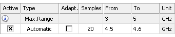
Multilayer Solver Overview

The multilayer Solver is a 3D planar electromagnetic solver for planar modeling and analysis. It is based on the Method of Moments (MoM) and enables users to simulate multilayer geometries accurately and efficiently. The solver features an automatic layer stack generation from a 3D model, automatic edge mesh refinement as well as an automatic de-embedding of ports. Accurate co-simulation together with CST DESIGN STUDIO for complex micro-strips and transmission lines in 2D becomes with the new multilayer solver easier than before, and together with CST's new System Assembly and Modeling (SAM) you can use the new solver to simulate planar components of complex systems now more efficiently.

Overview

Areas of application

Frequency sampling

Supported_materials

How_to_start_the_solver

Solver logfile

Areas of application

Typical applications are RF designs such as planar antennas and filters as well as MMIC and planar feeding network designs.

Frequency sampling

If you are interested in structure's S-parameters, the sampling method has a large influence on the calculation time. Automatically chosen frequency samples in conjunction with the broadband frequency sweep option usually will yield the broadband S-parameters with a minimal number of solver runs. Once the S-parameter sweep has finished, the solver can continue the S-parameter sweep just where it stopped, for instance in order to calculate additional samples, monitors, and further improve the sweep accuracy.

Example: A broadband frequency sweep with automatic sampling

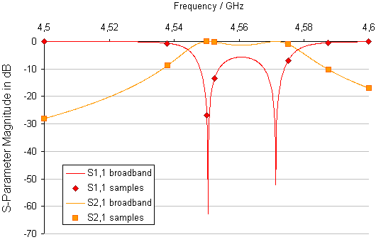
$image\Frequency_Domain_Sampling_Auto.png$

In this example seven frequency samples are calculated in a sub interval of the global frequency range. Please note that less than twenty samples are calculated, since the S-parameter convergence criterion is reached earlier.

You will see a quasi continuous curve when the broadband frequency sweep has been activated. The frequency samples are shown when Additional marks is checked in the 1D plot properties dialog, which can be invoked from the context menu when viewing S-parameters. If you deactivate the sweep in the Multilayer Solver Parameter dialog and press Apply, the samples which actually have been calculated will be shown as well, without the intermediate values.

$image\Frequency_Domain_S_Auto.png$

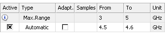
Example: A broadband frequency sweep with unlimited automatic sampling

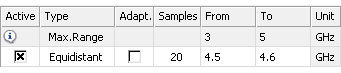
$image\Frequency_Domain_Sampling_AutoInf.png$

It is not necessary to define a maximum number of sample for the frequency sampling. When the number of samples is not defined (left blank) as shown above, the solver stops calculating additional samples as soon as the S-parameter sweep convergence criterion is satisfied. The results are the same as above, because the S-parameter sweep had converged after calculating seven frequency samples.

Example: A broadband frequency sweep with equidistant sampling

$image\Frequency_Domain_Sampling_Equidistant.png$

In this example twenty frequency samples are distributed equidistantly in a sub interval of the global frequency range with a frequency spacing of

$image\frequency_resolution.gif$

You will see a quasi continuous curve when the broadband frequency sweep has been activated. The frequency samples are shown when Additional marks is checked in the 1D plot properties dialog, which can be invoked from the context menu when viewing S-parameters. If you deactivate the sweep in the Multilayer Solver Parameters dialog and press Apply, the samples which actually have been calculated will be shown as well, without the intermediate values.

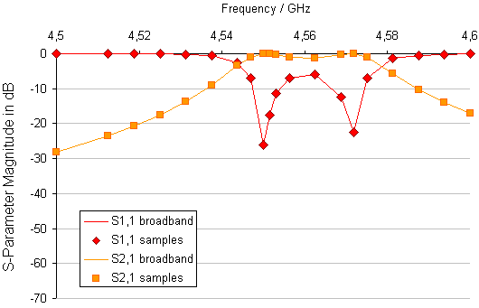
$image\Frequency_Domain_S_Equidistant.png$

Example: Automatic sampling without broadband sweep

$image\Frequency_Domain_Sampling_Auto.png$

Here twenty samples are calculated, but obviously more samples would be required to get an accurate representation of the S-parameter poles.

Please note that the broadband frequency sweep can be activated again after the simulation run in the Multilayer Solver Parameters dialog as a post processing step. Check the corresponding box and press Apply.

$image\Frequency_Domain_S_AutoOld.png$

Supported Materials

A wide range of material is supported by the multilayer solver.

PEC
anisotropic normal (loss free & lossy dielectrics) in the layer stackup
Lossy metal
Ohmic sheet
all electric frequency dependencies

For material information please see also Material Parameters.

How to start the solver

Before you start the solver you should make all necessary settings. See the Multilayer Solver Settings for details.

The multilayer solver can be started from the Multilayer Multilayer Solver Parameters dialog box.

Solver logfile

After the solver has finished you can view the logfile by choosing Post Processing: Manage Results Logfile . The logfile contains information about solver settings, mesh summary, solver results and solver statistics.