|
|
|
| 首页 >> CST教程 >> CST2013在线帮助系统 |
Rectangular Patch AntennaFrequency Domain Analysis Examples
General Description
This example shows a rectangular patch antenna. It demonstrates the usage of open boundary conditions for antennas and farfield monitors with the general purpose frequency domain solvers. The results are mainly focused on the farfield radiation pattern and S-parameters of the antenna. Furthermore, the "Calculate fields at axis marker" feature is used in a post-processing step. Like the tutorial example of a patch antenna this antenna can also be easily expanded into a patch antenna array. The structure has been simulated with the general purpose hexahedral and tetrahedral frequency domain solvers.
Structure Generation
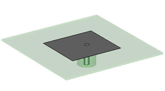
The structure can be defined using basic elements. The ground, the substrate and the patch shape are constructed with bricks. The inner feed and the inner conductor shape are cylinder shapes. Due to structure's symmetry a magnetic symmetry plane at the XZ plane can be introduced. Please note that this speeds up the solver, because only one half of the structure has to be calculated now, while the results remain exactly the same. The boundary condition was chosen to be open (add space) opposite to the ground plane and electric at the ground plane. The other boundary conditions are open. The advantage of the open (add space) boundary condition is that an adequate distance from the patch to the boundary is set automatically.
Parametrization
This example also demonstrates parametric construction. Therefore the following parameters have been defined:
It allows you to change the properties of the structure easily.
Note: When changing the y_shift parameter to a nonzero value, you also have to switch off the magnetic symmetry plane.
Mesh Settings (General Purpose Hexahedral Solver)
The mesh type was set to "Hexahedral Mesh" in the frequency domain solver dialog. The adaptive hexahedral mesh refinement was activated.
Solver Setup (General Purpose Hexahedral Solver)
In order to obtain the farfield radiation pattern a farfield monitor at the resonance frequency was defined. At the same frequency, E- and H-field monitors were defined. The adaptive hexahedral mesh refinement was activated. Since otherwise the default settings are used, the broadband frequency sweep is enabled.
Mesh Settings (General Purpose Tetrahedral Solver)
The mesh type remains "Tetrahedral Mesh"
in the frequency domain solver dialog. Curved elements in automatic mode are activated by default
(see Simulation:
Mesh
Solver Setup (General Purpose Tetrahedral Solver)
In order to obtain the farfield radiation pattern a farfield monitor at the resonance frequency was defined. The adaptive tetrahedral mesh refinement is activated by default. The adaptation frequency sample was moved to the monitor frequency (2.98 GHz). As an realization of the open boundary, PML has been selected in the solver specials.
Post Processing
The resulting scattering parameters can be accessed
through the 1D Results folder
in the navigation tree. Select 2D/3D
Results Details about the progression of the adaptive mesh
refinement are available in the navigation tree below 1D
Results Suppose you want to know the electric and magnetic
fields at a certain frequency when looking at the S-parameter 1D
Results
HFSS视频教程 ADS视频教程 CST视频教程 Ansoft Designer 中文教程 |
|
Copyright © 2006 - 2013 微波EDA网, All Rights Reserved 业务联系:mweda@163.com |
|