淘宝官方店推荐课程在线工具联系方式关于我们

	CST视频教程推荐 CST微波工作室入门与应用详解 \| CST使用操作基础

首页 >> CST教程 >> CST2013在线帮助系统

Dipole Antenna Array

Transient Analysis Examples - Antennas

Dipole Array, Combine Nearfield Results:
Dipole Array, Simultaneous Excitation:
Dipole Array, Farfield Array Feature:
Dipole Array, Combine Farfield VBA Feature:

$image\Dipole_Antenna_Array.gif$

General Description

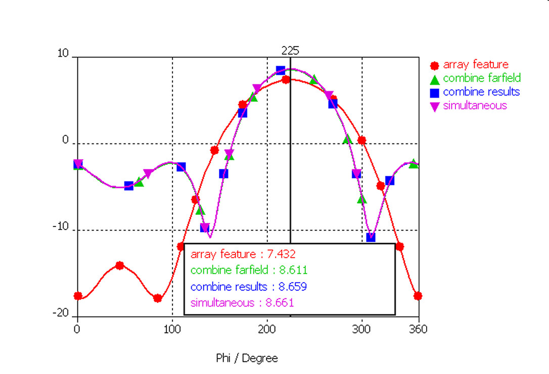
This example presents the farfield calculation of a planar 2x2 array pattern, consisting of four identical single electric dipoles, each holding a length of lambda/2 (lambda = 10 mm). Four examples show the behavior of this antenna pattern:

1. Combine Nearfield Results: The antenna's structure is generated as described below. Compared to the example Dipole Antenna here the complete array is modeled, the antennas separated in space by lambda/4 and showing a phase shift of 90 degree. Each dipole element is excited sequentially in four time domain simulation runs. In a post processing step, the superposition of the four results is calculated using the 'Combine Results...' feature considering a phase shift of 90 degree beween the single dipoles. Finally, the farfield is calculated from the combined result.

2. Simultaneous Excitation: The structure is the same as above in "Combine Nearfield Results", but the dipole elements are excited simultaneously with a phase shift of 90 degree between the single dipoles in one single time domain simulation run. This has the advantage of being four times faster, but the disadvantage, that the phase shift combination can not be modified quickly in post processing. Also, the given phase shift is only valid at one given frequency, because it has to be converted into a time shift for the simulation run.

3. Farfield Array Feature: The antenna is modeled as a single dipole element as described in the Dipole Antenna example. The array is calculated with the law of pattern multiplication, whereas the influence among the single array elements is neglected.

4. Combine Farfield VBA Feature: The structure is the same as above in "Combine Nearfield Results". Since the structure is rotationally symmetric, only port one is excited and the farfield for this stimulation is calculated. Afterwards, the resulting farfield is rotated and combined with phase shifts using a powerful VBA command. This way, the coupling of the array elements is taken into account, and the phase shift can still be modified without needing a time consuming solver run for recalculation. But still, only one time domain simulation run is necessary.

Structure Generation (of complete array)

One electric dipole is modelled by help of a single very thin cylinder consisting of PEC material, its dimensions are given parametrically. To provide some space for the location of the excitation source a small gap is cut in the antenna afterwards. Since the array pattern consists of identical elements, the single dipole is then multiplied to obtain the final structure using the transform feature with the copy option. Taking advantage of the given symmetry of the structure in z direction a corresponding electric x-y symmetry plane is defined.

Mesh Settings (of complete array)

Due to the structure's very small PEC elements it is necessary to refine the mesh in order to obtain results of sufficient accuracy. Therefore the number of mesh lines per wavelength is increased as well as the refinement factor at PEC edges. As a consequence the number of mesh nodes is increased.

Solver Setup (of complete array)

Before starting the simulation a farfield monitor is set at the respective frequency.

In order to enable a transient calculation, four discrete ports are defined as the excitation sources, feeding each of the electric dipoles. For the examples 1, 2 and 4, the simulation is then performed using the complete structure. For example 1, each antenna is stimulated separately, while for example 2, all antennas are excited simultaneously using an excitation list. For example 4, only port 1 is stimulated.

Post Processing

The previously defined farfield monitor offers now the possibility to investigate the radiation characteristics of the antenna array. The farfield results can be found in subfolders of the Farfields entry in the navigation tree.

In example 1 the radiation characteristics of each antenna as well as the behavior of the complete structure can be investigated. In addition, the nearfield effect of the antennas on each other can be examined regarding the scattering parameters concerning the different ports. The results of the four dipoles are combined to receive the overall farfield considering a phase shift of 90 degree between the antennas [1(1,90)+2(1,0)+3(1,-90)+4(1,0)] with the help of the Post Processing: 2D/3D Field Post Processing Combine Results option.

Example 2 allows the investigation of the farfield of the complete structure directly since all dipoles are excited simultaneously.

Example 3 offers the investigation of one single dipole as well as the farfield of the array. Here the influence among the single array elements is neglected. The array is calculated with the law of pattern multiplication. A 2x2 planar pattern is chosen perpendicular to the dipole axis, with a constant space shift of lambda/4 and a phase shift of 90 degree between the dipole elements.

For example 4 the project macro under Home: Macros Combine Farfields has to be run. It calculates the element farfield in 5 degree steps, combines the rotated element patterns and adds the combined pattern to the navigation tree. Note that in the VBA macro the positions of all four elements stay at zero, because the calculated array element farfield pattern has its farfield origin in the center of the whole structure and not in the center of element 1.

$image\Dipole_Antenna_Array_Result.jpg$

The farfield pattern results from all four examples are compared in example 4 under the navigation tree entry 1D Results Farfield Theta=90 using copy+paste. The plot shows the directivity in the x-y plane (theta=90deg.) over phi. The array behaves as a directional antenna with a main lobe at phi = 225 degree and a directivity of about 8.6 dB. The red curve which represents the array feature result of example 3, differs clearly from the other results. This effect is due to the negligence of the coupling between the array elements. Examples 1, 2 and 4 however are in perfect agreement with each other.

HFSS视频教程 ADS视频教程 CST视频教程 Ansoft Designer 中文教程


Copyright © 2006 - 2013 微波EDA网, All Rights Reserved 业务联系：mweda@163.com