|
|
|
| 首页 >> CST教程 >> CST2013在线帮助系统 |
Brick ResonatorEigenmode Analysis Examples
General Description
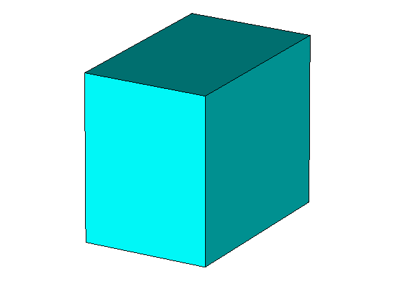
This example demonstrates a simple eigenmode calculation. The structure is a rectangular box with perfectly conducting walls and vacuum inside. Q-factors are calculated in the postprocessing step. The structure is used in four examples. Two of them use hexahedral mesh and the other two use tetrahedral mesh. The first and third example demonstrates the use of the optimizer together with the eigenmode solver.
Structure Generation
The background material is defined as perfectly conducting material, the units are changed to millimeters, gigahertz and nanoseconds, and the boundary conditions are set to "electric" in order to model perfectly conducting walls. The box resonator is created as a brick shape. Its dimensions are defined by three parameters (a, b and c), so that its geometry can be changed easily.
Solver Setup
When the eigenmode solver is started, a specific number of the lowest resonance frequencies of the structure is calculated. The relevant settings are defined using the default values, so that ten eigenmodes are considered.
Optimizer Setup (only for optimized brick)
The parameters considered for the optimization are listed here with its initial, minimum and maximum values:
Six samples are chosen, since the ranges of the values a, b, and c are rather wide. As optimizer type the Quasi-Newton optimizer with support of interpolation of primary data is chosen. The fundamental mode's frequency, which is supposed to be 10 GHz, is chosen as the first goal of the optimization. In order to increase the separation between the fundamental mode and the second mode, another optimizer goal is added: The frequency of mode 2 should exceed 14 GHz.
Post Processing
Non-optimized brick: The resulting mode information is listed in the navigation tree in the folder 2D/3D Results, subfolder Modes. Here the mode patterns as well as the corresponding eigenfrequencies can be found. The resonance frequencies are also stored in the logfile of the eigenmode solver. Depending on the dimensions of the box (a*b*c) the analytical solution of the problem can be written as f_res(m,n,o) = 0.5 * c * sqrt( (m/a)^2 + (n/b)^2 + (o/c)^2 ) (c = speed of light in the observed medium).
The default parameter settings (a = 13 mm, b = 17 mm and c = 20 mm) yield the following first three resonance frequencies:
The quality factors are calculated using 'Results/Loss and Q calculation'. For a conductivity of 5.8*10^7 S/m, the analytical values for mode one to three are given by
Optimized brick: After
the optimization process has finished, a new set of parameters is available.
From the results in the folders 2D/3D
Results
HFSS视频教程 ADS视频教程 CST视频教程 Ansoft Designer 中文教程 |
|
Copyright © 2006 - 2013 微波EDA网, All Rights Reserved 业务联系:mweda@163.com |
|