• 首页
• HFSS教程
• ADS教程
• CST教程
• 射频工程师培训
• 微波仪器使用培训
• 天线设计培训
• 射频专业基础课

Biological Tissue Voxel Model

Transient Analysis Examples - SAR Calculations

Thermal Solver Examples

This example is part of the CST MICROWAVE STUDIO examples and may not be present if these had been deselected during the installation process.

General Description

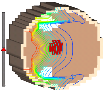
This example shows the Specific Absorption Rate (SAR) calculation and the use of the thermal solver with the bio-heat equation in biological tissue represented in a voxel model. A dipole is used for time domain excitation. The results of the transient high frequency solver run are used to perform the SAR calculation in a post processing step and as an excitation source for a following thermal solver run.

Note:

A very detailed human model data set is also available. Please contact CST.

Voxel Import

For the biological tissue data the voxel data import is used. In this example we use a very simple model without any third party copy right. It can easily be replaced by any other voxel model represented in a raw binary format with one byte per voxel. For this purpose, only the .vox and the material files in the Model\3D subdirectory of the project have to be adjusted to your models voxel resolution and material numbering with a text editor.

Mesh Setup

In order to easily control the mesh within the voxel model, a dummy brick of the same size is defined. Although the FPBA mesher does an accurate averaging of the voxel material data for any mesh, we define here as local mesh properties a maximum step of the same resolution as the voxel model which is 2mm.

HF Solver Setup

Before starting the transient solver the dipole with a discrete port as excitation source has to be defined and monitors have to be set for power loss density and e-field at the frequency of interest.

Post Processing

The SAR calculation is based on the power loss density monitor. It can be started through the Post Processing: 2D/3D Field Post processing SAR dialog box. In this example we have defined a template under Post Processing: Result Templates Results Template Based Post Processing 0D Results which is automatically executed after the solver run. After the SAR calculation is finished the results are accessible via the 2D/3D Results SAR folder in the navigation tree. Detailed SAR results like Total SAR are available via Context menu Object Properties... when the 3D result is selected in the navigation tree.

Thermal Solver Setup

To receive a temperature distribution and other thermal results, the thermal solver can be run using the power loss density of the HF EM solver as a heat source. Therefore, first set the problem type to thermal by selecting Home: Simulation Problem Type Thermal. Menus and ribbons are reconfigured and we can define an excitation by Home: Sources and Loads Thermal Losses . In the dialog box we set the source field, a power scaling factor of 1 and activate the option Consider electric volume losses. Please note that the thermal conductivity and the heat capacity for the background material and 'Air' have been set before the HF solver run.

Before starting the thermal solver we make sure that in the solver dialog box special settings the bio-heat equation is active and the blood temperature is appropriately set to 37 degree Celsius.

                HFSS视频教程                                      ADS视频教程                               CST视频教程                           Ansoft Designer 中文教程

      Copyright © 2006 - 2013   微波EDA网, All Rights Reserved    业务联系：mweda@163.com