|
|
|
| �� | |
| �� | |
| ��ҳ >> CST�̳� >> CST2013���߰���ϵͳ |
Magnetic Resonance ImagingTransient Analysis Examples - SAR CalculationsThermal Solver Examples
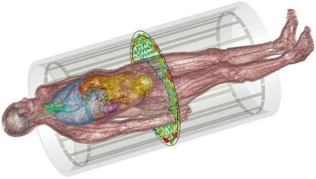
There are two versions of this example. The first contains a human model of the CST Voxel Family and needs a special license to be loaded. The second example contains just the empty MRI coil. For disk space reasons the full 2D/3D results are not provided for these examples, but they can be easily obtained by just starting the transient solver and then the thermal solver as described in the Thermal Solver Setup paragraph below. We thank the Institute of Biometrics and Medical Informatics, Otto von Guericke University Magdeburg, Germany for generously providing the MRI coil setup. Both examples are part of the CST MICROWAVE STUDIO examples and may not be present if these had been deselected during the installation process. General Description Magnetic Resonance Imaging (MRI) uses the magnetic moments of protons to generate detailed 3D pictures of the inside of the human body for medical purposes with relatively low side-effects. The procedure involves strong magnetic fields at different frequencies and with different orientations, which implies quite a challenge for the design of the device. First of all a very strong static magnetic field aligns all magnetic moments in the body. For the MRI device used in this example this biasing magnetic field strength is 1.5 Tesla, which is a typical value for clinical MRI devices. The nuclear resonance itself is excited at the protons intrinsic resonance of 63 MHz (dependent on the static field) with a magnetic field rotating around the axis of the magnetostatic axis (z-axis in this example). The field generating so-called ”body-coil” is supposed to offer a homogeneous field distribution all over the body. Finally additional gradient coils, operating in the kHz range, are used for the positioning the point of resonance inside the body. Solver Set-up This simplified example only focuses on the RF part at 63 MHz in the body-coil and uses the transient solver of CST MICROWAVE STUDIO. The other aspects of MRI can be tackled with the magnetostatic solver or the magneto-quasistatic solver of CST EM STUDIO. The model consists of a cylindrical ground plane and a typical bird-cage coil. Lumped capacitors are used to tune the coil to the required 63 MHz. The coil is driven by two discrete ports positioned at a 90° angle, which excites the required rotating field. This could be done by two separate runs followed by a combine results operation or �?as in this example �?by a simultaneous excitation of both ports with a 90° phase shift. Post-Processing The main design goal of an RF body coil for MRI
is the homogeneity and the rotating character of the magnetic field. This
so-called H1+ field (or B1+ in case of µr
= 1) can be obtained running the macro Home:
Macros Additionally, potential health hazards need to be investigated. This can be done either by evaluating the Specific Absorption Rate (SAR) or by directly calculating the body temperature using the stationary bio-heat solver inside the CST MPHYSICS STUDIO for a ”worst case” estimation. In both cases, results were scaled to a typical excitation power of 50 W rms. Standardization requires the SAR value to be below 10 W/kg averaged over 10g cubes or the body temperature increase to be below 1°C. See below the rotating H field in the cross section shown in the first figure, and the 3D SAR distribution as well as the temperature in Kelvin in a cross section in the center of the human model. Thermal Solver Setup To obtain a temperature distribution and other thermal
results, a thermal solver run can be applied using the power loss density
of the HF EM solver as a heat source. Therefore, first set the problem
type to thermal using Home:
Simulation Before starting the thermal stationary solver please assure that in the solver dialog box special settings the bio-heat equation is active and the blood temperature is appropriately set to 37 degree Celsius.
HFSS��Ƶ�̳� ADS��Ƶ�̳� CST��Ƶ�̳� Ansoft Designer ���Ľ̳� |
�� |
|
Copyright © 2006 - 2013 ��EDA��, All Rights Reserved ҵ����ϵ��mweda@163.com |
|