![]()
![]()
|
Single Run: |
|
Geometric Construction and Solver Settings
Introduction and Model Dimensions
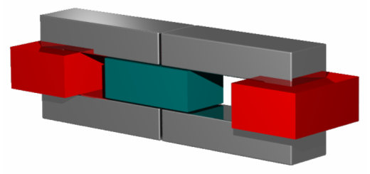
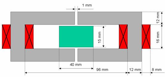
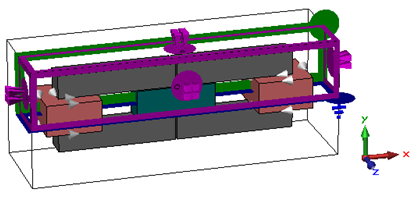
In this tutorial, you will run a magnetostatic simulation with a subsequent force calculation. The examined model is a linear motor consisting of two coils, two iron yokes and a permanent magnet. The yokes form a magnetic circuit that is driven by coils with currents of opposing polarity. A current-dependent force is then exerted on a movable permanent magnet located between the yokes. After the construction steps have been completed, you will perform the necessary solver settings and start a first simulation. Finally, the force calculation and the parameter sweep feature are explained to check the linearity of the device.
We strongly suggest that you carefully read through the CST EM STUDIO Workflow & Solver Overview manual before starting this tutorial.
After launching the CST STUDIO SUITE you will enter the
start screen showing you a list of recently opened projects and allowing
you to specify the application which suits your requirements best. The
easiest way to get started is to configure a project template which sets
the basic settings that are meaningful for your typical application. Therefore
click on the Create Project ![]() button in the New Project
section.
button in the New Project
section.
Next you should chose the application area, which is Statics and Low Frequency for the example in this tutorial and then select the workflow by double-clicking on the corresponding entry.
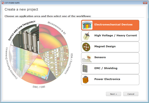
For the linear motor, please select Electromechanical
Devices ![]() Actuators
Actuators ![]() M-Static
M-Static
![]() .
.
At last you are requested to select the units which fit your application best. The linear motor device in this tutorial has dimensions given in mm. Therefore select mm from the Dimensions drop-down list. For the specific application in this tutorial the other settings can be left unchanged. After clicking the Next button, you can give the project template a name and review a summary of your initial settings.
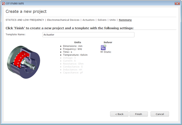
Finally, click the Finish button to save the project template and to create a new project with appropriate settings. CST EM STUDIO will be launched automatically due to the choice of the application area Statics and Low Frequency.
Please note: When you click again on File: New and Recent you will see that the recently defined template appears below the Project Templates section. For further projects in the same application area you can simply click on this template entry to launch CST EM STUDIO with useful basic settings. It is not necessary to define a new template each time. You are now able to start the software with reasonable initial settings quickly with just one click on the corresponding template.
Please note:
All settings made for a project template can be modified later on during
the construction of your model. For example, the units can be modified
in the units dialog box (Home:
Settings ![]() Units
Units ![]() ) and the solver type can be selected in the Home:
Simulation
) and the solver type can be selected in the Home:
Simulation ![]() Start Simulation drop-down list.
Start Simulation drop-down list.
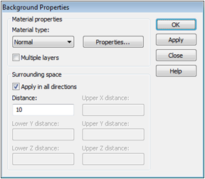
Once you have entered the modeling view, the background
properties should be adjusted. Because the structure will be defined in
a vacuum background, you must define the size of the surrounding empty
space. Therefore, select Modeling:
Materials ![]() Background
Background ![]() to enter the Background
Properties dialog box. The selected project template has already
set the Material
type to Normal and Distance of 10 mm to the calculation domains boundaries for each direction.
This is completely fine for our purposes. Therefore, confirm these settings
by pressing the OK button.
to enter the Background
Properties dialog box. The selected project template has already
set the Material
type to Normal and Distance of 10 mm to the calculation domains boundaries for each direction.
This is completely fine for our purposes. Therefore, confirm these settings
by pressing the OK button.
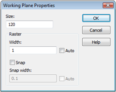
The next step will usually be to set the working plane
properties in order to make the drawing plane large enough for your device.
Because the structure has a maximum extension of 120 mm along a coordinate
direction, the working plane size should be set to at least 120 mm. These
settings can be changed in a dialog box that opens after selecting View:
Visibility
![]() Working Plane
Working Plane ![]() Working Plane Properties
Working Plane Properties ![]() .
.
Furthermore, de-select the Auto and Snap check-boxes for both raster settings before pressing the OK button.
The first step for the linear motor is the construction
of the first yoke. For this purpose, the extrude tool must first be used.
Please activate the extrusion mode by selecting Modeling:
Shapes ![]() Extrude
Extrude ![]() . When you are prompted to pick the first polygon point, you
can also enter the coordinates numerically by pressing the Tab
key.
. When you are prompted to pick the first polygon point, you
can also enter the coordinates numerically by pressing the Tab
key.
In this case, you should enter 9 points defining the polygon that will be extruded to form the first yoke. Please press the Tab key and enter the first point's coordinates as X = 0.5 and Y = 8 in the dialog box and press the OK button. Afterwards, you can repeat these steps for the second point:
Press the Tab key
Enter X = 0.5, Y = 20 in the dialog box and press OK.
Repeat this procedure for all points from the following list:
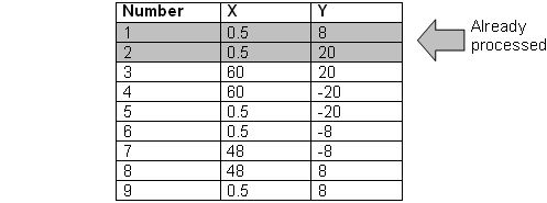
After you have entered the last point, you will be requested to enter the height of the extrude body.
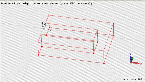
This can also be accomplished numerically by pressing the Tab key again, entering the Height of 12 and pressing the OK button. Now the following dialog box will appear, displaying a summary of your previous input:
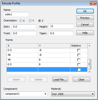
Please check all these settings carefully. If you encounter any mistakes, please change the value in the corresponding entry field.
You should now assign a meaningful name to the extrude body by entering e.g. yoke1 in the Name field. Finally, you need to define the yoke's material. Because no material has yet been defined for the yoke, you should open the material definition dialog box by selecting [New Material...] from the Material drop down list. In this dialog box you should
define a new Material name (e.g. Iron 1000),
set the Type to a Normal material,
change the permeability constant Mue to 1000,
and choose a color for the material by pressing the colored button.
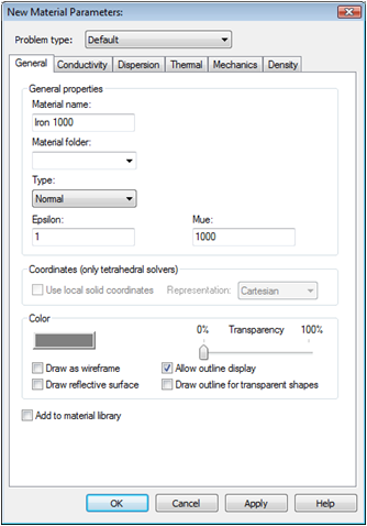
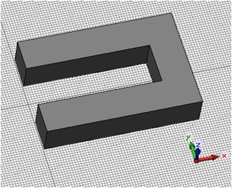
Finally, pressing the OK button. Back in the extrude creation dialog box you can also press the OK button to create the first yoke. Your screen should now appear as follows (you can press the Space key in order to zoom the structure to the maximum possible extent):
The next construction step deals with the definition
of the second yoke using the transform tool. Select the first yoke by
double-clicking on it or selecting its tree item in the navigation tree.
Then select Transform from the
context menu or from the ribbon Modeling:
Tools ![]() Transform
Transform ![]() to open the Transform
dialog box. Select the Mirror
operation and enter an X-value
of 1 for the Mirror
plane normal. To create a transformed copy of the first yoke, check
the Copy box.
to open the Transform
dialog box. Select the Mirror
operation and enter an X-value
of 1 for the Mirror
plane normal. To create a transformed copy of the first yoke, check
the Copy box.
![]()
To obtain a graphical feedback for your input you might use the Preview button.
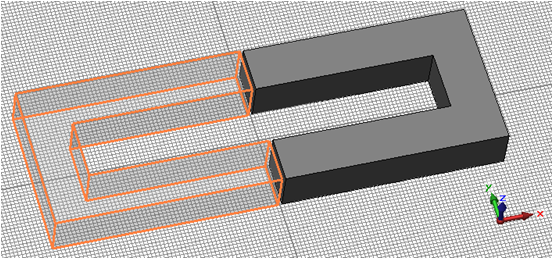
Finally press OK to create the second yoke. To change the name of the second yoke, select its item in the navigation tree and select Rename from the context menu (or press F2). Now the item text inside the tree becomes editable and you should assign a more suitable name to the new solid (e.g. yoke2).
The geometric definition of the permanent magnet can
be easily accomplished with the brick tool. Please activate the brick
creation mode by clicking on the corresponding icon (Modeling:
Shapes ![]() Brick
Brick ![]() ). You will be asked to enter the first point
of the base rectangle. Similar to the extrude tool, you may enter the
values with the mouse by double-clicking at the desired position, or numerically
by pressing the Tab key. Define
the brick with
). You will be asked to enter the first point
of the base rectangle. Similar to the extrude tool, you may enter the
values with the mouse by double-clicking at the desired position, or numerically
by pressing the Tab key. Define
the brick with
the first point at X = -20, Y = -7.5.,
the second point at X = 20, Y = 7.5,
a height of 12.
In the Brick dialog box assign a Name to the brick (e.g. magnet) and define a new material for the magnet. Therefore, select [New Material...] from the Material
drop down list to enter the material dialog box again. The magnet will be made of Normal material with Epsilon and Mue values of 1. Choose an appropriate name (e.g. magnet material) and color for the new material and then leave the dialog box by pressing the OK button.
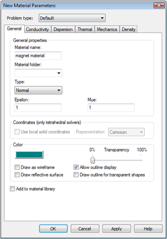
You will return to the brick dialog box which you can also leave with the OK button.
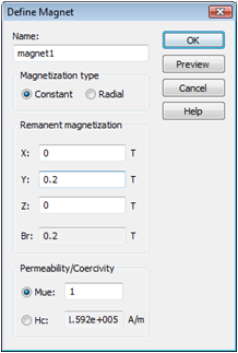
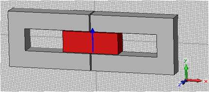
Now define the permanent magnet's magnetization vector.
To this end, activate the permanent magnet tool by selecting Simulation:
Sources and Loads
![]() Permanent Magnet
Permanent Magnet ![]() . When asked to select the magnets surface,
move the mouse cursor to the previously defined brick and select it with
a double-click. The selected surface will be highlighted red and the Magnet dialog box will open. Enter
0.2 for the Y-component of the
magnetization vector. Pressing the Preview
button shows you the orientation of the current magnetization vector.
For this example, the approximate Permeability
value 1 can be left unchanged.
. When asked to select the magnets surface,
move the mouse cursor to the previously defined brick and select it with
a double-click. The selected surface will be highlighted red and the Magnet dialog box will open. Enter
0.2 for the Y-component of the
magnetization vector. Pressing the Preview
button shows you the orientation of the current magnetization vector.
For this example, the approximate Permeability
value 1 can be left unchanged.
|
|
|
To store your settings, press OK. The permanent magnet definition can always be reviewed by selecting its icon in the Permanent Magnets folder of the navigation tree.
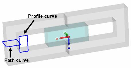
The final step in the construction process of the linear
motor is the creation of the two coils. The coils dimensions are defined
by a profile curve and a path curve. Therefore, you must define curves
before you activate the coil tool. The coil's profile is a rectangle.
Therefore, select Simulation:
Curves ![]() Curves
Curves ![]() Rectangle
Rectangle ![]() . Use the Tab
key for numerical input of the coordinates. Define
. Use the Tab
key for numerical input of the coordinates. Define
the first point at X = 40, Y = -8 and
the second point at X = 48, Y = 8.
The Rectangle dialog box will open. Confirm your settings with OK.
To define the path curve you have to activate the working
coordinate system (WCS) by selecting Simulation:
WCS ![]() Local WCS
Local WCS ![]() . After its activation, the WCS is
still aligned with the global coordinate system. In this case, the WCS
has to be rotated around the u-axis by +90 degrees. To do this, you can
use the shortcut Shift+u or select
Simulation:
WCS
. After its activation, the WCS is
still aligned with the global coordinate system. In this case, the WCS
has to be rotated around the u-axis by +90 degrees. To do this, you can
use the shortcut Shift+u or select
Simulation:
WCS ![]() Transform WCS
Transform WCS ![]() , activate the Rotate
option and enter the Angle 90
in the U edit field.
, activate the Rotate
option and enter the Angle 90
in the U edit field.

The coil's path curve is a rectangle as well. Select
the rectangle tool again (Simulation:
Curves ![]() Curves
Curves ![]() Rectangle
Rectangle ![]() ) and define
) and define
the first corner at U = 47, V = -1 and
the second corner at U = 61, V = 13
Finally, in the rectangle dialog box confirm the settings by pressing the OK button.
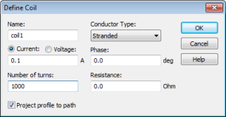
Now it is time to define the first coil. Select Simulation:
Sources and Loads
![]() Coil
Coil ![]() to activate the coil creation mode. You will be requested to
select the coil's profile curve. Select the first rectangle (as shown
in the above picture) with a double-click. Next,
you have to select the coil's path curve with a double-click to open the
coil dialog box with a preview. Enter a current Value
of 0.1 A and the Number
of turns as 1000. Confirm
with OK.
to activate the coil creation mode. You will be requested to
select the coil's profile curve. Select the first rectangle (as shown
in the above picture) with a double-click. Next,
you have to select the coil's path curve with a double-click to open the
coil dialog box with a preview. Enter a current Value
of 0.1 A and the Number
of turns as 1000. Confirm
with OK.
|
|
|
The second coil can be created by simply mirroring the first one. Therefore, select the previously defined coil and activate the Transform dialog box by selecting Transform from the context menu of from the Modeling ribbon. Set the Operation type to Mirror and the Mirror plane normal to U = 1. To create a transformed copy of the coil, check the Copy checkbox. Then, perform the transformation with the OK button.
|
|
|
Finally, change the name of the second coil as done before with the yoke: Select its item in the navigation tree and choose Rename from the context menu (or press F2) to make the tree item editable. Enter an appropriate name (e.g. coil2) and confirm by pressing the Enter key.
Congratulations! The geometric construction is now completed. Before the simulation can be started, however, several solver settings must be applied.
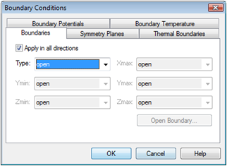
The calculation domain is covered and terminated by six faces, to each of which a boundary condition must be assigned. In fact, the influence of the boundary conditions for this calculation is rather small because the magnetic flux density is mainly focused inside the iron core of the structure. However, as previously mentioned, the structure is embedded in a vacuum atmosphere and therefore all boundary conditions should be set to type open.
Enter the Boundary
Conditions dialog box by selecting Simulation:
Settings ![]() Boundaries
Boundaries ![]() . Activate the Apply
in all directions checkbox and select open
from the Type drop-down list.
You will recognize that the modeler view also changes according to the
currently set boundary conditions:
. Activate the Apply
in all directions checkbox and select open
from the Type drop-down list.
You will recognize that the modeler view also changes according to the
currently set boundary conditions:
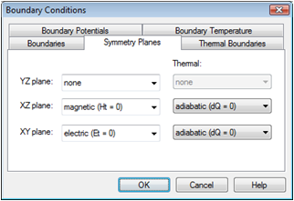
Obviously, the structure is symmetric with respect to the XY- and XZ-planes. To save simulation time you can define symmetry conditions that need to suit the field inside these planes. Please click on the Symmetry Planes tab in the Boundary Conditions dialog box and set the symmetry of the XZ plane to magnetic (Ht = 0) and the XY symmetry to electric (Et = 0).
The magnetic boundary condition sets the tangential component of the magnetic field to zero; it behaves like a perfect magnetic conductor (PMC). In contrast, the electric boundary forces the normal component of the magnetic flux density to be zero; it appears to be like a perfect electrical conductor (PEC). The table below shows the conditions for different field types at these boundary / symmetry conditions:
|
|
Magnetic boundary |
Electric boundary |
|
Electric field / flux |
D-normal = 0 |
E-tangential = 0 |
|
Magnetic field / flux |
H-tangential = 0 |
B-normal = 0 |
|
Stationary current |
J-normal = 0 |
J-tangential = 0 |
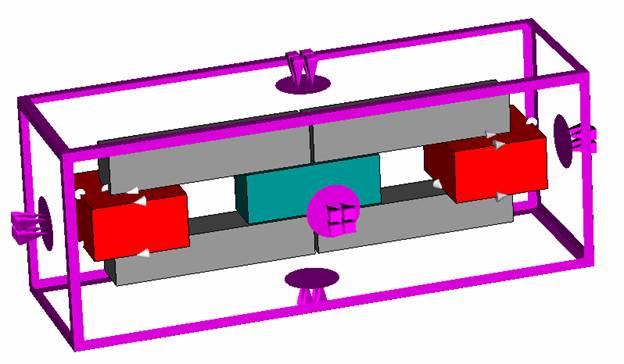
While the Symmetry Planes tab is active, the Modeler View displays the currently set symmetry planes. Back in the Boundaries tab, the given boundary conditions are visualized as well:
The blue-framed plane indicates a magnetic and the green-framed plane an electric symmetry setting in the screenshot above. The pink ones correspond to the open boundary conditions. Finally close the dialog box with the OK button.
Disclaimer: Please note that setting the XZ symmetry plane will cut the calculation domain parallel to the coil windings. This may cause minor differences to calculations without symmetry planes because the internal representation of the current paths inside the coil will change slightly.
For the numerical solution of a field problem, it is
necessary to discretize its calculation domain. This means that the volume
will be subdivided, or in other terms, that a mesh will be placed on the
structure. CST EM STUDIO supports two strategies: tetrahedral and hexahedral
meshes. It this tutorial, the hexahedral grid will be employed. Therefore,
select Home:
Mesh ![]() Global Properties
Global Properties ![]() Hexahedral
Hexahedral ![]() from the drop-downlist. The Mesh
Properties dialog box will open with the Hexahedral
settings. The project template has set the Lower
mesh limit to 20 and the Mesh
line ratio limit to 50. Confirm the settings by pressing OK. CST EM STUDIO then automatically
generates a calculation mesh that can be modified by the user in many
ways.
from the drop-downlist. The Mesh
Properties dialog box will open with the Hexahedral
settings. The project template has set the Lower
mesh limit to 20 and the Mesh
line ratio limit to 50. Confirm the settings by pressing OK. CST EM STUDIO then automatically
generates a calculation mesh that can be modified by the user in many
ways.
To take a first look at the automatically generated mesh,
activate the Mesh view (![]() ).
).
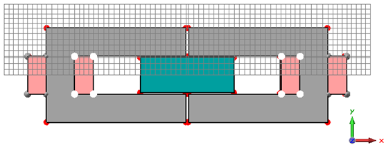
The picture above shows the z-meshing plane at the position
z = 6, i.e. the first meshed plane in z-direction. You can obtain the
same view if you activate the z-meshing plane by clicking on the Z Normal (![]() ) button or by just typing Z.
You can use the tools in the Mesh Plane
group to switch to another mesh plane normal (
) button or by just typing Z.
You can use the tools in the Mesh Plane
group to switch to another mesh plane normal (![]() ,
, ![]() ,
, ![]() ) or to vary the displayed mesh plane (
) or to vary the displayed mesh plane (![]() ,
,
![]() ).
).
In our case, the automatically generated mesh is still quite coarse at the air gap between the yokes and the magnet. To get accurate results, it is necessary to refine the mesh inside the air gaps. A finer mesh leads to a more accurate field calculation inside the gaps and increases the accuracy of the subsequent force computation.
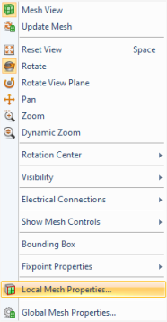
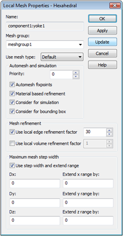
To refine the mesh inside the air gaps, select yoke1 and open the Local Mesh Properties dialog box which is accessible via the context menu:
|
|
|
Because the mesh needs to be refined in the yokes' surroundings, you need to specify an edge refinement factor that allows a better sampling of the air gaps. Activate the local edge refinement by marking the checkbox and set the edge refinement factor to a value of 30.
Please note that this high refinement factor only takes effect because the Mesh Line Ratio Limit inside the global mesh properties dialog box has been set to a very high value of 50 by the magnetostatics template.
When you press OK
a new mesh group appears in the navigation tree in the folder Groups
![]() Mesh Groups. This mesh groups is called meshgroup1
as specified in the previous dialog box. To apply the same local mesh
setting to the second yoke, simply drag its item in the navigation tree
(Components
Mesh Groups. This mesh groups is called meshgroup1
as specified in the previous dialog box. To apply the same local mesh
setting to the second yoke, simply drag its item in the navigation tree
(Components ![]() component1
component1 ![]() yoke2) to the folder Groups
yoke2) to the folder Groups
![]() Mesh Groups
Mesh Groups ![]() meshgroup1. Examination of the mesh reveals that the
transitions between the yokes and the surrounding air have been refined:
meshgroup1. Examination of the mesh reveals that the
transitions between the yokes and the surrounding air have been refined:
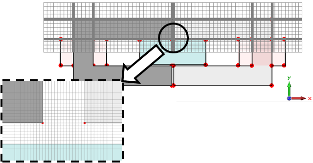
Obviously, the mesh is now strongly refined within the
gap areas of the structure. Finally, leave the Mesh
View by toggling Mesh: Close ![]() Close Mesh View
Close Mesh View ![]() .
.
The solver parameters are specified in the magnetostatic
solver control dialog box that can be opened by clicking on Simulation:
Solver ![]() Start Simulation
Start Simulation ![]() . Please set the Accuracy
to 1e-4 and start the solver
with the Start button.
. Please set the Accuracy
to 1e-4 and start the solver
with the Start button.

After CST EM STUDIO has calculated the magnetic field
and magnet flux density, the force on the magnet can be calculated. Therefore,
switch back to the global WCS (deactivate Simulation:
WCS ![]() Local WCS
Local WCS ![]() ). Then select Post Processing:
2D/3D Field Post
Processing
). Then select Post Processing:
2D/3D Field Post
Processing ![]() Forces
Forces ![]() to open the Calculate
Force and Torques dialog box.
to open the Calculate
Force and Torques dialog box.
Because we are not interested in any torques here, just press the Calculate button to start the force calculation. The forces on all solids will now be calculated. After the calculation has finished, a result window opens containing forces and torques on every solid. To close this window, press the OK button. This window can be reopened at any time by selecting the MForces entry in the navigation tree.
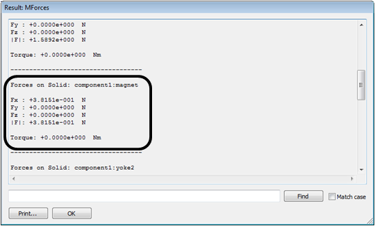
Please note that the results might differ slightly depending on the operating system and the architecture of the machine with which they were computed.
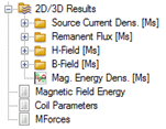
Congratulations, you have simulated the linear motor! Let's examine the calculated fields. You will notice that some new entries have appeared in the Navigation Tree:
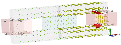
As mentioned above, this tutorial focuses on the force
applied to the magnet. In addition, the magnetic field and the flux density
are available. The following screenshot shows the magnetic flux density
distribution (B-Field) in the
entire calculation domain. Due to the magnetization of the permanent magnet,
the flux density is significantly larger in the right yoke than in the
left one. To get a better view, you can enter the Plot
Properties via the context menu or by selecting 2D/3D Plot:
Plot Properties ![]() Properties
Properties ![]() and modify
the Objects (i.e. arrows). Maybe
you want to increase the arrows' density, scale them or activate a logarithmic
scaling.
and modify
the Objects (i.e. arrows). Maybe
you want to increase the arrows' density, scale them or activate a logarithmic
scaling.
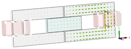
This plot gives you a first impression about the fields
in and around the magnetic circuit. For a more detailed analysis, activate
the 2D plot in a plane by selecting 2D/3D Plot:
Sectional View ![]() 3D Fields on 2D Plane
3D Fields on 2D Plane ![]() .
.
Again it is possible to modify plot settings by selecting Plot Properties from the context menu. For more information on this subject please refer to the Online Help.
One of the most advanced features of CST EM STUDIO is the parameterization ability. This means that you can define variables and use them, for instance, for the definition of a solid. The solver contains the option to vary parameters within a user-defined range. 1D Results will be summarized in tables and can be plotted as a function of the varied parameters.
The built-in Parameter Sweep tool is explained in detail in the CST EM STUDIO Workflow & Solver Overview manual. In this section only the main steps to set up a parameterized project for the Parameter Sweep are described.
Because a linear dependency between the force on the magnet and the coil driving currents is desired, the current definitions for the coils, made in the previous chapter, will be controlled by a parameter. Select the first coil item in the navigation tree and select Edit Coil Properties from its context menu. In the corresponding dialog box, replace the Value 0.1 by a new variable (e.g. current). Confirm with OK (delete the results if required) and enter the value 0.1 for the newly defined parameter. Apply the same steps to the second coil to change its current definition:
Select the second coil in the navigation tree
Open the Edit Coil Properties dialog box in the context menu
Replace the old current definition by the name of the previously defined variable current.
To start the parameter sweep, enter the magnetostatic
solver dialog box first (Simulation:
Solver ![]() Start Simulation
Start Simulation ![]() ) and press the Par.
Sweep button to get to the Parameter
Sweep dialog box. Here you can define a new sequence and a parameter
to sweep (e.g. sweep the current
from 0 to 1 in 6 samples). Moreover you should define the result of interest.
Therefore, click on the Result Template...
button. The Template Based Postprocessing
dialog box will appear, where you can select the template folder Statics and Low Frequency and the postprocessing
step Calculate Force and Torque.
) and press the Par.
Sweep button to get to the Parameter
Sweep dialog box. Here you can define a new sequence and a parameter
to sweep (e.g. sweep the current
from 0 to 1 in 6 samples). Moreover you should define the result of interest.
Therefore, click on the Result Template...
button. The Template Based Postprocessing
dialog box will appear, where you can select the template folder Statics and Low Frequency and the postprocessing
step Calculate Force and Torque.
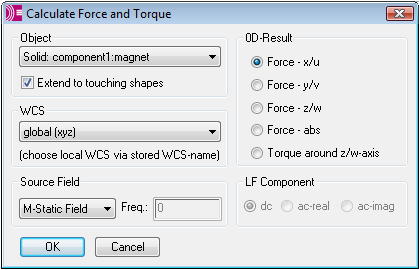
Another dialog box will open requiring the settings for the force calculation. Here select the magnet (component1:magnet) from the Object drop-down list and the x/u component of the Force in the 0D-Result frame. Furthermore, make sure that the M-Static Field is selected in the Source Field frame. The other settings can be left unchanged.
Confirm these settings by pressing the OK
button and leave the Template Base Postprocessing
dialog box with the Close button.
Back in the Parameter Sweep dialog
box, press Start to run the simulation.
Finally, after the parameter sweep has finished, close the dialog box
with the Close button and examine
the result of the parameter sweep by Tables
![]() 0D Results
0D Results ![]() Force_x_magnet in the navigation tree.
Force_x_magnet in the navigation tree.
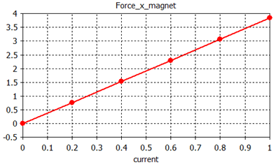
The force on the magnet has a linear dependency on the current inside the coils.
A static field calculation is mainly affected by two sources of numerical inaccuracies:
Numerical errors introduced by the iterative linear equation system solver.
Inaccuracies arising from the finite mesh resolution.
In this section we provide hints on how to minimize these errors and achieve highly accurate results.
CST EM STUDIO uses an iterative linear equation system solver to solve the discretized field problem. This means that the iterative solver will stop a calculation if a given accuracy has been reached. In most cases, an accuracy setting of 1e-6 is sufficient. However, for some problems with very high material or mesh ratios, the solver will give you a warning that some results are inaccurate and that you should consider increasing the solver accuracy.
Inaccuracies arising from the finite mesh resolution are usually more difficult to estimate. The only way to ensure the accuracy of the solution is to increase the mesh resolution and recalculate the results. When they no longer significantly change as the mesh density is increased, then convergence has been achieved.
In the example above, you have used a modified default
mesh. The easiest way to test the accuracy of the results is to use fully
automatic mesh adaptation that can be switched on by checking the Adaptive mesh refinement option in
the solver control dialog box (Simulation:
Solver ![]() Start Simulation
Start Simulation ![]() ). Improve the Accuracy
setting to a value of 1e-6 to
avoid numerical problems. Run the solver again by pressing the Start button.
After the mesh adaptation procedure
). Improve the Accuracy
setting to a value of 1e-6 to
avoid numerical problems. Run the solver again by pressing the Start button.
After the mesh adaptation procedure
has finished, you can visualize the energy error for
two subsequent passes by selecting 1D
Results ![]() Adaptive Meshing
Adaptive Meshing ![]() Error from the navigation tree:
Error from the navigation tree:
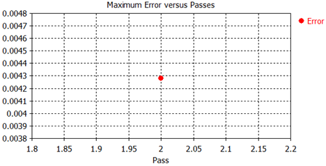
Within two passes, the mesh adaptation was able to reduce the energy error below the requested limit. As you can see, the maximum energy deviation between the first and second passes is already below 0.5%, indicating that the calculation with the first mesh produced quite accurate results. A final look on the forces calculated with the adapted mesh shows that the absolute force deviation on the magnet is also below 0.5%.
Congratulations! You have just completed the linear motor tutorial that should have provided you with a good working knowledge on how to use the magnetostatics solver. The following topics have been covered:
General modeling considerations, using templates, etc.
Model a linear motor by using the extrude, the brick and the transformation tool.
Define a permanent magnet.
Define coils.
Define boundary and symmetry conditions.
Modify the automatically generated mesh.
Start the magnetostatics solver.
Visualize the magnetic fields.
Use the force calculation.
Perform a parameter sweep.
Obtain accurate and converged results using the automatic mesh adaptation.
You can obtain more information for each particular step from the online help system that can be activated either by pressing the Help button in each dialog box or by pressing the F1 key at any time to obtain context sensitive information.
In some instances we have referred to the CST EM STUDIO Workflow & Solver Overview manual that is also a good source of information for general topics. In addition to this tutorial, you can find additional magnetostatic calculation examples in the Examples folder in your installation directory. Each of these examples contains a Readme item in the navigation tree that will give you more information about the particular device.
And last but not least: Please also visit one of the training classes regularly held at a location near you. Thank you for using CST EM STUDIO.