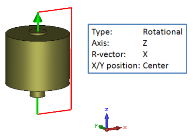
This example shows how to simulate a linear actuator within the 2D magnetostatic solver. Nonlinear material properties are applied to the steel parts. The structure is driven by a current coil, consisting of 100 turns, each carrying a current of 5 A. The dimensions of the model are fully parameterized and thus can be changed easily to perform different calculations. The parameter for the airgap can be used to compute the force vs. position characteristic in a parameter sweep.
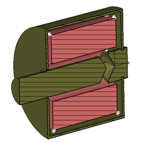
The actuator consists of three cylinders with nonlinear material properties (Steel ST37). A nonlinear material is defined by its B-H curve, which can be entered manually in the nonlinear tab of the layer dialog. Alternatively it is possible to import data from an Ascii file or to use material data from the built-in material library.
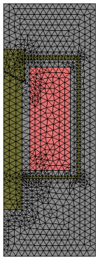
Due to the axis-symmetric structure, the 2D rotational mesh can be applied.
The 2D rotational symmetric tetrahedral solver is started with default settings and the adaptive mesh refinement. Since the initial mesh contains less than 2000 triangles the whole nonlinear simulation takes only a few seconds including the mesh adaptation process.
|
|
|
|
Initial 2D mesh |
Adapted 2D mesh |
After the calculation has finished the computed energy and co-energy as well as the flux linkage is available in the Navigation Tree. One can view the mu distribution inside the nonlinear material by selecting the "2D/3D Results/Material" entry in the navigation tree and switching to "inside" in the plot properties. Furthermore, you can activate "Draw 3D fields on 2D plane" to visualize the material distribution and other field quantities on a cutting plane. A postprocessing template computes the force on the armature.
With choosing ‘Par. Sweep’ in the solver dialog box the force vs. position curve can be simulated.
This example shows how to simulate nonlinear material properties within the magnetostatic solver. The structure is driven by a current coil, consisting of 2500 turns, each carrying a current of 10 A. The dimensions of the model are fully parameterized and thus can be changed easily to study variations of the geometry.