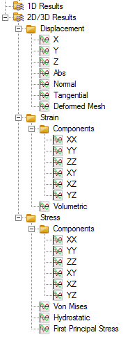

The mechanical solver creates all results automatically after the simulation process was finished. This means it is not necessary to define any monitors in advance.

Displacement
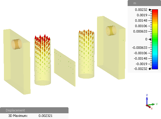
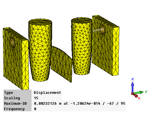
The stationary displacement distribution is a vector 3D field which can be evaluated also on a 2D cut-plane. Another possibility to visualize the displacement field is to switch to the Deformed Mesh plot by selecting "2D/3D Results\Displacement\Deformed Mesh" in the Navigation Tree.


Strain
The strain distribution is a 2nd rank symmetric tensor field. In the linear solver, the strain tensor is defined as follows:

Here ui represent the components of displacement vector and xi the coordinates. Single components of the strain tensor can be visualized as scalar plots. Besides, the volumetric strain representing the relative volume change in each point of the solution domain is calculated as the trace of the strain tensor.
Stress
The mechanical stress is a 2nd rank symmetric tensor field. In the linear solver case, the stress tensor is linearly dependent on strain:

Single components of the stress tensor can be visualized as scalar plots. Besides, the following scalar stress fields are calculated:
Von Mises stress can be used as a yield criterion by comparing it to the yield strength of the material.
Hydrostatic stress, or "pressure", is the average of the diagonal elements of the stress tensor.
First principal stress is the maximal eigenvalue of the stress tensor representing the maximal tension acting in the point.
Besides, imported fields such as temperature or force densities are visualized, which makes it possible to estimate the quality of interpolation.
See also
Mechanical Solver Overview, Post Processing Overview, Template Based Post Processing