Farfield View

The different farfield monitors are listed in the Navigation Tree, indicated by their names and their respective excitation port number in square brackets.

In each subfolder, different farfield views are available depending on the chosen polarization, the plot mode and the farfield calculation method. On the left-hand side, two examples of a navigation tree with different farfield views are shown.

Applying Plot properties... in the context menu leads you to the corresponding Farfield Plot Dialog, also available using Farfield Plot: Plot Properties Properties.

All farfield plots are presented in the main plot window, where some relevant farfield characteristics, such as radiation or total efficiency in the case of 2D and 3D plots, are shown in the window’s lower left corner. See further information on the special farfield conventions in the Farfield Overview.

Different settings regarding quality, scaling and various plot types (polar and cartesian plots as well as 2D and 3D graphics) or modes (directivity, gain, electric or magnetic field or power pattern) are available in the Farfield Plot Dialog. In addition, the orientation and origin of the coordinate system as well as different field components may be selected in this dialog box. Furthermore, the Farfield Array Dialog enables the calculation of specified array patterns based on the selected farfield monitor.

To get the raw plot data in ASCII format, use Export Plot Data (ASCII).

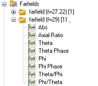
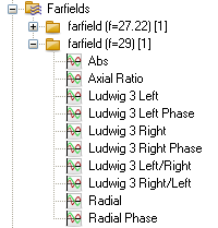
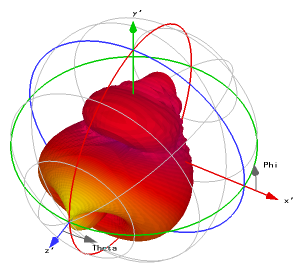
For each farfield, the absolute value of the field components is available through the Navigation Tree entry ”Abs.” The different field components that may be plotted depend on the chosen polarization. This can be either the normal linear polarization, circular polarization or slant polarization. The entries in the Navigation Tree correspond to the coordinate system as shown in the figure above. Sample 3D plots for these coordinate systems are listed below.

If the farfield is calculated without the farfield approximation, the radial farfield component is calculated as well and can be accessed through the Navigation Tree.

Furthermore, it is possible to plot the phase of a field component if the plot mode is set to ”E-Field” or ”H-Field” . In this case, an additional entry appears in the Navigation Tree allowing to plot the phase of each field component. All other plot mode settings display the phase of the corresponding E-field component.

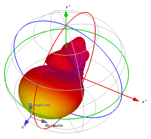
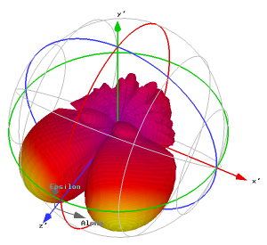
The following table shows four plots of the same farfield represented in different coordinate systems. The ETheta, EElevation, EAlpha and EVertical components are displayed in the spherical, "Ludwig 2 Azimuth over Elevation", "Ludwig 2 Elevation over Azimuth" and the "Ludwig 3" coordinate systems, respectively. In addition, iso longitude and latitude lines (see Farfield Plot - General) are plotted in gray to highlight the location and orientation of the chosen coordinate system and the proper angles.


(a) ETheta (Spherical coordinate system)	(b) EElevation (Ludwig 2, Azimuth over Elevation)

(c) EAlpha (Ludwig 2, Elevation over Azimuth)	(d) EVertical (Ludwig 3)

Farfield View

In the farfield view, all relevant components concerning previously defined farfield monitors are visualized and can be changed.

The different farfield monitors are listed in the Navigation Tree, indicated by their names and their respective excitation port number in square brackets.

In each subfolder, different farfield views are available depending on the chosen polarization, the plot mode and the farfield calculation method. On the left-hand side, two examples of a navigation tree with different farfield views are shown.

Applying Plot properties... in the context menu leads you to the corresponding Farfield Plot Dialog, also available using Farfield Plot: Plot Properties Properties.

To get the raw plot data in ASCII format, use Export Plot Data (ASCII).

If the farfield is calculated without the farfield approximation, the radial farfield component is calculated as well and can be accessed through the Navigation Tree.

Farfield View

In the farfield view, all relevant components concerning previously defined farfield monitors are visualized and can be changed.

The different farfield monitors are listed in the Navigation Tree, indicated by their names and their respective excitation port number in square brackets.

In each subfolder, different farfield views are available depending on the chosen polarization, the plot mode and the farfield calculation method. On the left-hand side, two examples of a navigation tree with different farfield views are shown.

Applying Plot properties... in the context menu leads you to the corresponding Farfield Plot Dialog, also available using Farfield Plot: Plot Properties Properties.

To get the raw plot data in ASCII format, use Export Plot Data (ASCII).

If the farfield is calculated without the farfield approximation, the radial farfield component is calculated as well and can be accessed through the Navigation Tree.

Applying Plot properties... in the context menu leads you to the corresponding Farfield Plot Dialog, also available using Farfield Plot: Plot Properties Properties.