|
微波射频仿真设计 |
|
|
微波射频仿真设计 |
|
| 首页 >> Ansoft Designer >> Ansoft Designer在线帮助文档 |
|
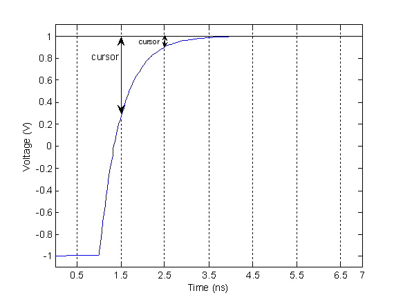
Nexxim Simulator > VerifEye AnalysisVerifEye analysis is a statistical eye-analysis algorithm, similar to the public domain StatEye (see QuickEye and VerifEye References for a citation).VerifEye calculates a cumulative distribution function (CDF) for deviations from the step responses in the intermediate waveform described above, taking into account the conditional probabilities for the various kinds of transitions. A slice through the CDF generates the bathtub curve. Moreover, random transmit jitter can be simulated by using a Gaussian distribution for the deviations in response. VerifEye analysis uses the edges for calculations (rather than the pulses as in standard StatEye). Using the edges allows random jitter to be truly random (timings of edges are independent) and also enables an easy calculation of duty cycle distortion (DCD). The idea behind VerifEye is that in order to generate an eye diagram and bathtub curve for a channel, including the effects of jitter, it is not necessary to run a very long transient simulation, such as would be implied by the required BER of the channel. By combining the statistics of the bit stream with the variation in transitions due to jitter, it is possible to generate the information needed in much less computation time. First, consider a particular point on the QuickEye waveform described above. That point is the sum of all the voltage excursions caused by the various transitions from high to low or low to high at bit interfaces before the time point in question. It is here that we can apply the statistical concept. Rather than calculating the voltage excursions for all possible combinations of bits, we can calculate a probability distribution for the sum of all the excursions. Perhaps it is easiest to consider this concept in terms of what are known as “cursors”; the deviations from the ideal waveform.
Figure 5: The two largest cursors from the step response of the RC example. If the channel were perfect, then the response would be identical to the input; the voltage at each point in time would be either +1V or -1V, depending on the bit in question. Referring to Figure 5, imagine what the waveform would look like if there were a very large number of 1s in a row, versus a large number of 0s, followed by a transition to a 1. In the first case, the waveform would have time to settle to its correct final value of +1V. In the second case, the waveform would be in transition from -1V to +1V because of imperfections in the channel. The difference between those two waveforms is a “cursor”, as shown in Figure 5. Now, let us explore how we might calculate the intersymbol interference statistically. Let us assume that the current bit is a 1. This can happen in two ways: either the previous bit was a 1, in which case there was no transition between them, or the previous bit was a 0, in which case there was a low-to-high transition between them. The probability of a transition is 0.5, if the bits are independent. In the first case, the cursor is zero; in the second case, it has some significant negative value, corresponding to the slow rise time of the step response at the end of the channel. Statistically, therefore, the waveform has a 50% chance of having no deviation, and a 50% chance of having a negative deviation equal to the cursor value. It is clear that we can chain this process forward and backward, considering each “postcursor” and precursor in turn. The primary difficulty is that, even if the bits are independent, the transitions are not; a high-to-low transition cannot be followed by another high-to-low transition; there must be a low-to-high transition in between. However, this constraint can be handled by the appropriate application of conditional probabilities. What results from all of the above are probability distribution functions (PDFs) for the voltage value of the waveforms of high and low bits. These functions can be combined into cumulative distribution functions (CDFs), contours of which give the traditional eye diagram. Another measure of the signal integrity of a channel is the “bathtub curve”. This is a measure of the width of an eye opening at a certain level, usually halfway between the high and low levels. The bathtub curve turns out to be particularly easy to generate using statistical methods: it is simply a slice through the CDF determined above.
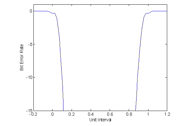 Figure 6: Bathtub curve for RC example, with 10ps random transmit jitter. X axis is time; Y axis is common logarithm of BER.
HFSS视频教程 ADS视频教程 CST视频教程 Ansoft Designer 中文教程 |
|
Copyright © 2006 - 2013 微波EDA网, All Rights Reserved 业务联系:mweda@163.com |
|